Abstract—The early exercise property of American option changes the original Black-Scholes equation to an inequality that cannot be solved via traditional finite difference method. Therefore, finding the early exercise boundary prior to spatial discretization is a must in each time step. This overhead slows down the computation and the accuracy of solution relies on if the early exercise boundary can be accurately located. A simple numerical method based on finite difference and method of lines is proposed here to overcome this difficulty in American option valuation. Our method averts the otherwise necessary procedure of locating the optimal exercise boundary before applying finite difference discretization. The method is efficient and flexible to all kinds of pay-off. Computations of American put, American call with dividend, American strangle options are demonstrated to show the efficiency of the current method.
Index Terms—American option, finite difference method, method of lines, American put option, American call option with dividend, American strangle option
I. INTRODUCTION
N last two decades, the problem of pricing American options has been investigated extensively both in numerical methods and analytical approximations. These two approaches both encounter the arduous challenge which is known as a free boundary value problem arising form the early exercise feature of American options. The difficulty associated with the valuation of American options stems from the fact that the optimal exercise boundary must be determined as a part of the solution. Unfortunately, the early exercise boundary cannot be solved in a close form, and, consequently, nor can the option’s value. Up to now, reviewing all relevant literatures, most efforts have been exerted mainly on locating the free boundary that sets the domain for the Black-Scholes equation.
For analytic approximations, Johnson [19] adopted an interpolation scheme to price the American put option for a non-dividend paying stock. MacMillan [22] used a quadratic approximation, which involved solving an approximate partial differential equation (PDE) for the early exercise premium, the amount by which the value of an American option exceeds a European one, to evaluate an American put
Manuscript received March 10, 2013; revised April 7, 2013. This work was supported in part by the Taiwan National Science Council under Grant NSC-101-2115-M-035-001.
T.-L. Horng is a professor of the Department of Applied Mathematics, Feng Chia University, Taichung, Taiwan 40724 (corresponding author to provide phone: 886-922263146; fax: 886-424510801; e-mail: tlhorng123@ gmail.com).
C.-Y. Tien was with Department of Mathematics, University of York, Heslington, York, UK. He is now a quantitative analyst at Royal London Asset Management, 55 Gracechurch St, City of London, Greater London, EC3V 0UF (e-mail: [email protected]).
option. Geske and Johnson [15] obtained a valuation formula for American put option expressed in terms of a series of compound-option functions. Following [22], Ju and Zhong [20] presented an efficient and accurate approximate formula for pricing American options on a dividend paying stock.
For numerical approximations, the most popular numerical methods for pricing American options can be classified to lattice method, Monte Carlo simulation and finite difference method. Sure, besides finite difference methods, there are other popular numerical method based on discretization for solving PDEs like finite element method, boundary element method, spectral and pseudo-spectral methods and etc. Here we just use finite difference to stand for methods of this kind. In fact, finite difference method ranks as the most popular one among its kind in financial engineering. The lattice method is simple and still widely used for evaluating American options. It was first introduced by Cox et al. [9], and the convergence of the lattice method for American options is proved by Amin and Khanna [1]. The Monte Carlo method is also popular among financial practitioners. It is appealing, simple to implement for pricing European options, and especially has advantage of pricing multi-asset options. For pricing American options, Monte Carlo method requests some further modification due to the early-exercise feature. Fu [13], [14] priced American-style options by using Monte Carlo method in conjunction with gradient-based optimization techniques. Duck et al. [11] proposed a technique which generates monotonically varying data to enhance the accuracy and reliability of Monte Carlo-based method in handling early exercise features.
The application of finite difference method to price American options can be first found in [4], [5], [26]. Jaillet et al. [18] showed the convergence of the finite difference method. A comparison of different numerical methods for American options pricing was discussed in [6], [16]. Generally, there still exist some difficulties in using these numerical methods. For finite difference method, the difficulty arises from the early exercise property, which changes the original Black-Scholes equation to an inequality that cannot be solved via traditional finite difference process. Therefore, finding the early exercise boundary prior to spatial discretization (discretization on underlying asset) is a must in each time step. This overhead slows down the computation and the accuracy of solution relies on if the early exercise boundary can be accurately located. For lattice method and Monte Carlo simulation, although they do not have the free boundary value problem, they would need some extra efforts to compute the Greeks and the optimal exercise boundary, which are mostly desired in practice besides option valuation. In this paper, we propose a simple numerical method based on finite difference method and method of lines (MOL)
A Simple Numerical Approach for Solving
American Option Problems
Tzyy-Leng Horng and Chih-Yuan Tien
to overcome the difficulty mentioned above in American option valuation. Particularly, our method averts the otherwise necessary procedure of locating the optimal exercise boundary before applying finite difference discretization. This method is efficient, flexible to all kinds of pay-off, and easy to implement when compared with many other methods. The results also show that our method possesses the optimal accuracy intrinsic to finite difference discretization, and thereby make it a powerful tool for practitioners when evaluating American option and financial derivatives having American option feature.
This paper is organized as follows. Section II is devoted to the description of method of lines. Section III describes the core idea of our scheme of evaluating American option through the spirit of Black-Scholes inequality with demonstrations through successful computation of American put, American call with dividend, and American strangle options. Optimal accuracy is also shown in these examples. Section IV depicts the scheme of locating the optimal exercise boundary. The dual optimal exercise boundaries in American strangle option are particularly compared with Chiarella and Ziogas [7], and satisfactory agreement is observed. Section V makes the conclusion by emphasizing the merits of the current method.
II. METHOD OF LINES
Under the usual assumptions, Black and Scholes [2] and Merton [23] have shown that the price V of any contingent claim written on a stock, whether it is American or European, satisfies the famous Black-Scholes equation:
2 2 2
2
1
(
)
0
2
V
V
V
S
r D S
rV
t
S
S
, (1)where volatility σ, the risk-free rate r, and dividend yield D
are all assumed to be constants. The value of any particular contingent claim is determined by the terminal and boundary conditions. For an American option, notice that the PDE only holds in the not-yet-exercised region. At the place where the option should be exercised immediately, the equality sign in (1) would turn into an inequality one. That means the option value V(S,t) at each time follows either V(S,t)=f(S,t) for the
early exercised region or 2
2 2 2 1
( ) 0
2
V V V
S r D S rV
t S S
for the
not-yet-exercised region, where f(S,t) is the payoff of an American option at time t. There is a moving boundary that separates these two regions and makes the whole problem a free boundary problem for Black-Scholes equation. Generally, this early exercised boundary is difficult to locate and there is no simple closed-form expression for it. Most finite difference methods nowadays exert their efforts on locating the early exercise boundary that is a must before finite difference discretization can be applied to the not-yet-exercised region.
The method of lines (MOL), a popular method for solving PDEs in engineering, was first promoted by Liskovets [21]. The idea is first reducing a time-dependent PDE to a system of ordinary differential equations (ODEs) in time via semi-discretization in space. Then this system of ODEs in time can further be solved efficiently by many well-developed ODE solvers. This methodology has been successfully applied to the valuation of American options on
common stock, and is found to be accurate and efficient [8], [17], [24]. To explain how MOL is employed, here we simply take valuation of a European call as an example. Incorporating with 2nd order finite difference scheme, we can
discretize (1) on a uniform mesh of underlying asset price
0N i i
S into a semi-discrete system of ODEs in time:
dV
idt
1
2
2
S
i
2
V
i1
2
V
i
V
i1
S
2
(
r
D
)
S
iV
i1
V
i12
S
rV
i,
i
1,...,
N
1.
, (2)
The boundary conditions of equation (1) are
( , )
1, as
, 0
,
(0, ) 0, 0
.
V S t
S
t T
S
V
t
t T
Both boundary conditions above exhibit linear behavior close to boundaries, and hence they can be incorporated into this system of ODEs by neglecting the 2nd order derivative in S,
and compensating 1st order derivative in S with 2nd order
accurate, one-sided difference approximation
0 0 1 2
0 0
3
4
(
)
,
2
dV
V
V V
r D S
rV
dt
S
(3)1 2
3
4
(
)
,
2
N N N N
N N
dV
V
V
V
r D S
rV
dt
S
(4)for (2) with S being truncated to Smax which is specified
by Smax=3K or Smax=4K considering both computational
efficiency and acceptable boundary error. Equations (2-4), symbolically denoted as , pose as an ordinary differential initial value problem in time and can be solved by many efficient ODE solvers which have been developed in hundreds of years. Actually, traditional finite difference method incorporating with explicit Euler scheme in time integration is equivalent to choose forward Euler scheme as the ODE solver in MOL. Likewise, popular Crank-Nicolsen finite difference scheme is equivalent to select the Adams-Moulton one-step method (trapezoidal rule) as the ODE solver in MOL. As noted in [24], the free boundary initially moves with infinite speed but slows down very quickly. Therefore, this stiff problem would be hard to implement efficiently by plain finite difference methods. To evaluate American option efficiently, it would request a self-adjusting-in-time-step solver for time integration, and this can be done easily by novel ODE solvers nowadays featuring self-adjusting variable step size and order (VSVO). Many VSVO type ODE solvers have been collected in popular MATLAB® ODE suite. In the current study, we
selected ode23 from the suite to be our demonstrating ODE solver. Ode23 implements an explicit Runge-Kutta (2,3) pair developed by Bogacki and Shampine [3]. It features by an adaptive step size controlled by specified error tolerance and is an efficient on-step solver for moderately stiff ODE’s. More details of this solver can be found in [3].
III. VALUATION OF AMERICAN OPTIONS
all finite difference methods for pricing American options, including those employing MOL mentioned above, request to find out the optimal exercise boundary first in each time step. This procedure is a must, and accurate location of this optimal exercise boundary is crucial to the overall accuracy. That is why many analytical mathematicians study this subject and compete on deriving a better analytic approximation of optimal exercise boundary that is crucial to finite difference methods.
However, our current method does not request this optimal exercise boundary at all in each time step, and this optimal exercise boundary can be extracted from the numerical results afterwards if wanted. Due to the saving of overhead on computing this optimal exercise boundary, our method is much more efficient compared with other numerical methods. The key idea of our method is to modify (2-4) to
, 0 ,
0,1, … , .
(5)This idea is based on the fact that the value of an American option, when evolving backward in time, can not allow smaller than its final pay-off at any time before expiration. If it is smaller than its final pay-off, the option should then be early exercised at that spot. This spirit can also be observed in evaluating American options by binomial tree. To elaborate our point, for those nodes i that do not need early exercise, their option values would be governed by the backward time evolution of Black-Scholes equation and
, 0
.
For option values at other nodes i that would fall below their final pay-off if following the backward evolution of Black-Scholes equation, it would request an early exercise and then
, 0
0.
Equation (5) actually can deduce the Black-Scholes inequality for American options:
2 2 2
2
1
(
)
0.
2
V
V
V
S
r D S
rV
t
S
S
Solving (5) is straight forward and easy to implement in the frame work of MOL. Extracting the optimal exercise boundary, if wanted, can be done afterwards from the result by re-computing dVi/dt, for all i at each time step, and locating the single zero of dVi/dt through interpolation. This trajectory of single zero would be the optimal exercise boundary. The details of computing this optimal exercise boundary will be discussed in a later section below. Actually, this idea can be implemented by conventional finite difference techniques such as forward Euler and Crank-Nicolsen methods too. We can simply integrate the Black-Scholes equation backward in time at each time step, and then replace the option value falling below the final
pay-off by it at those nodes that need an early exercise. This can be justified rigorously by thinking of Black-Scholes inequality above as Black-Scholes equation with an additional a priori unknown forcing function. The only purpose of this forcing function is to make sure that, once the prices at those nodes fall below the pay-off when evolving backward in time, the forcing function will compensate those prices to become the pay-off value. One may still argue about the adoption of this unknown a priori forcing function, and this can be justified by the governing equation (6) for American put option shown below. We can see the option price retains its continuity in both the function itself and its spatial derivative all the time at the interface (the early exercise boundary) and then for the whole domain [0,Smax].
This implies the existence of a forcing function that is non-zero only on those early-exercised nodes. Though forward Euler or Crank-Nicolsen finite difference scheme may then look like a simpler way to evaluate American options by adopting the idea above, however, as mentioned before, the free boundary moves extremely fast near the expiry date, which would request much finer mesh in time near the expiry date. This makes these two conventional finite difference techniques with fixed time step very inefficient to reach small time error near the expiry date. If the mesh of time is not appropriately resolved near the expiry date, it may cause large errors in both the option value and optimal exercise boundary. Under this situation, MOL employing VSVO-type error-control ODE solvers would be a much more superior method. Also, the current method agrees with the spirit of linear complementarity. Here, we use American put option, American call option with dividend and American strangle option to demonstrate how our simple approach would work.
A. American Put Option
Here the optimal exercise boundary Sf,P(t) separates the underlying asset domain in two regions, continuation and stopping regions. On the stopping region [0, Sf,P(t) ×[0,T],
V(S,t)=KP-S, while on the continuation region [Sf,P(t),∞ ×[0,T], V(S,t) needs to satisfy the following free-boundary problem:
V
t
1 2
2
S22V
S2(rD)S
V
S rV0,
Sf,P(t)S, 0tT,
V(S,T)max(KPS,0), S0,
V S
f,P(t),t
KPSf,P(t), 0tT, limSSf,P(t)
V
S 1, 0tT,
Sf,P(T)min KP,rKP D
.
(6)
Naturally, finding out the optimal exercise boundary would be a must before integrating (6). Instead, our simple method solves (5) with linear boundary conditions (3-4) and the terminal condition V(S,T)=max(KP-S,0). The specific parameter values adopted here in our computation are
from S=0 to S=1 with the infinite domain of S being truncated by five times of the exercise price KP. The error analysis of our result is reported in Table I. The first part in this table lists the calculated option price at the exercise price. For calculating absolute error, we calculated a binomial tree with exhaustive N=10,000 time steps and used the result as the exact solution Vexa(Si,0). Here, we again limit the maximum time step to be 10-4 so that the total error would be dominated
only by the spatial error. The column of absolute error again shows perfect 2nd order convergence. In the second part, the
maximum absolute error (MAE),
0
max ( ,0)i exa( ,0)i
i NV S V S
,
shows that the order of accuracy deteriorates slightly from 2nd
order, and the location of MAE is mostly close to the free boundary except at N=400, in which the location of MAE is close to exercise price. This deterioration may be due to the fact that V fails to twice differentiable at the optimal exercise boundary. As we know, error analysis of finite difference is based on Taylor expansion. 2nd order of accuracy on the
whole range of S would request the justification of twice differentiability on all S. As to the computed free boundary, from Table I, it seems to converge in first-order sense without rigorous analysis provided here.
B. American Call Option with Dividend
The optimal exercise boundary Sf,C(t) separates the underlying asset domain to continuation and stopping regions. On the stopping region (Sf,C(t), ∞ ×[0,T],
V(S,t)=S-KC, while on the continuation region [0,Sf,C(t)]×[0,T], V(S,t) needs to be solved from the following free-boundary problem for American call options:
V
t
1 2
2S22V
S2(rD)S
V
S rV0,
0<S<Sf,C(t), 0tT,
V(S,T)max(SKC,0), S0,
V S
f,C(t),t
Sf,C(t)KC, 0tT, limSSf,C(t)
V
S 1, 0tT,
Sf,C(T)min KC,rKC D
.
(7)
The above opting pricing problem can be solved exactly in the same way as pricing American put option before only with the terminal condition changed to V(S,T)=max(S-KC,0). Table II reports the error analysis of American call option pricing. The specific parameter values are r=9%, σ=40%,
D=10%, T=1, KC=1/5, and stock price ranges from S=0 to
S=1. Same as before, the infinite domain of S is truncated by five times of the exercise price KC. The first part in this table lists the calculated option price at the exercise price. Again, for calculating absolute error, we calculated a binomial tree with exhaustive N=10,000 time steps and used the result as the exact solution. Here, both the local error at the exercise price and MAE show perfect 2nd order of convergence, with
MAE happening near exercise price instead of optimal exercise boundary as happening above in the case of American put.
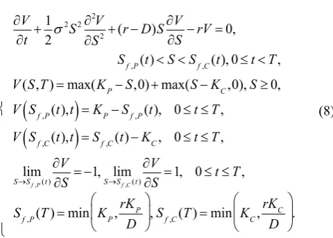
C. American Strangle Option
To demonstrate the flexibility of our method that can be applied to any kind of pay-off function, here we apply our method to the option pricing of an American strangle position, unusually seen on the market, studied first by Chiarella and Ziogas [7]. American strangle pay-off can be comprehended as a combination of American put and call, and there would be two free boundaries when option evolves backward in time. The optimal exercise boundaries Sf,P(t) and
Sf,C(t) separates the underlying asset domain into continuation and stopping regions. On the stopping region [0, , ×[0,T], V(S,t)=KP-S, and (Sf,C(t), ∞ ×[0,T],
V(S,t)=S-KC, while on the continuation region (Sf,P(t),Sf,C(t))×[0,T], V(S,t) is governed by the following free-boundary problem for American strangle:
V
t
1 2
2S22V
S2(rD)S
V
S rV0,
Sf,P(t)SSf,C(t), 0tT,
V(S,T)max(KPS,0)max(SKC,0),S0,
V S
f,P(t),t
KPSf,P(t), 0tT,V S
f,C(t),t
Sf,C(t)KC, 0tT, limSSf,P(t)
V
S 1, limSSf,C(t)
V
S 1, 0tT,
Sf,P(T)min KP,rKP
D
,Sf,C(T)min KC,rKC
D
.
(8)
Though the pay-off of American strangle is a combination of put and call positions, its current value would not just be the sum of the associated American put and call. This is chiefly because the dual optimal exercise boundaries, Sf,P(t) and
Sf,C(t), are not independent. Chiarella and Ziogas [7] first derived a set of complicated coupled integral equations for these dual early exercise boundaries. Then they solved the Black-Scholes equation for the option value in the continuation region by Crank-Nicolsen finite difference method. Using our simple method, it needs only to change the terminal condition to be the following pay-off function
[image:4.595.307.547.242.413.2]V(S,T)=max(KP-S,0)+max(S-KC,0), and follow the procedure same as above.
Table III reports our result of American strangle pricing. The parameter values r=5%, σ=20%, D=10%, T=1, KP=1,
N=800 results almost match with every digit of the exact solutions that used N=120,000 space nodes in [7]. We conclude that our simple method can be easily and robustly applied to all kinds of pay-off functions and have a satisfactory accuracy with an economic spatial resolution.
IV. ESTIMATING THE OPTIMAL EXERCISE BOUNDARY Different from other methods, the optimal exercise boundary is not requested at each time step for our method. However, it can be extracted from the numerical result afterwards if wanted. We first re-compute dVi/dt, for all i at each time step by (2). Then the optimal exercise boundary Sopt
would be the single zero of , =0 as mentioned before. Instead of doing time-consuming root finding, Sopt can be simply interpolated by dVi/dt. The way is to see S as function of ⁄ instead, since ⁄ vs. Si is monotonic across
Sopt. We can then interpolate to find Sopt through Si vs.
⁄ . There are other more accurate ways of locating
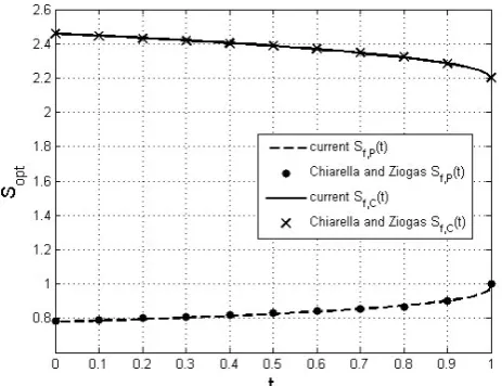
Sopt like utilizing Delta value for example. Taking American put as an example, we can extrapolate to find Sopt that approximates , 1 through Si vs. ⁄ in the continuation region near optimal exercise boundary. Fig. 1 shows the dual optimal exercise boundaries Sf,P(t) and
Sf,C(t) of the American strangle option in Table III. To demonstrate the accuracy of locating optimal exercise boundary by the current method, we particularly computed the dual optimal exercise boundaries Sf,P(t) and Sf,C(t) with
r=10%, σ=20%, D=5%, T=1, KP=1, KC=1.1, as in Figs. 2 and 3 of [7] and the comparison is shown in Fig. 2. Obviously, our result agrees very well with [7].
V. CONCLUSION
We have introduced an efficient numerical method to evaluate American options in this article. This simple method is much easier to implement compared with those numerical methods requesting the early exercise boundary calculated in advance at each time step. Not requesting the early exercise boundary makes it flexible to suit all kinds of pay-off function. The optimal exercise boundary can be easily extracted afterwards from the computed option values at each time step if wanted. Various ways like interpolating on the Theta or Delta values can do the purpose efficiently. This efficient method can be directly extended to evaluate many more general American option problems such as two-factor American option [12], [25], and two-factor convertible bond with embedded call and put options [10]. Also, tracing their optimal exercise boundaries/regimes afterwards is easy by current method no matter how complicated those early-exercised constraints would be.
REFERENCES
[1] K. Amin, and A. Khanna, “Convergence of American option values from discrete to continuous time financial models,”Mathematical Finance, vol. 4, pp. 289–304, 1994.
[2] F. Black, and M. Scholes, “The pricing of options and corporate liabilities,” Journal of Political Economy, vol. 81, pp. 637-654, 1973.
[3] P. Bogacki, and L. F. Shampine, “A 3(2) pair of Runge-Kutta formulas,”
Applied Mathematics Letters, vol. 2, pp. 1-9, 1989.
[4] M. Brennan, and E. Schwartz, “The valuation of American put options,”
Journal of Finance, vol. 32, pp. 449–462, 1977.
[5] M. Brennan, and E. Schwartz, “Finite difference methods and jump processes arising in the pricing of contingent claims: a synthesis,”
Journal of Financial and Quantitative Analysis, vol. 13, pp. 461–474, 1978.
[6] M. Broadie, and J. Detemple, “American option valuation: new bounds, approximations, and a comparison of existing methods,” Review of Financial Studies, vol. 9, pp. 1211–1250, 1996.
[7] C. Chiarella, and A. Ziogas, “Evaluation of American strangles,”Journal of Economic Dynamics and Control, vol. 29, pp. 31-62, 2005.
[8] P. Carr, and D. Faguet, “Fast accurate valuation of American options,”
unpublished.
[9] J. C. Cox, S. A. Ross, and M. Rubinstein, “Option pricing: a simplified approach,”Journal of Financial Economics, vol. 7, pp. 229–263, 1979.
[10] J. de Frutos, “A finite element method for two factor convertible bonds,
” in Numerical Methods in Finance, M. Breton, and H. Ben-Ameur, Ed. Springer, 2005, pp. 109-128.
[11] P. W. Duck, D. P. Newton, M. Widdicks, and Y. Leung, “Enhancing the accuracy of pricing American and Bermudan options,” Journal of Derivative, vol. 12, pp. 34-44, 2005.
[12] G. E. Fasshauer, A. Q. M. Khaliq, and D. A. Voss, “Using mesh free approximation for multi-asset American option problems,”Journal of Chinese Institute of Engineers, vol. 27, pp. 563-571, 2004.
[13] M. C. Fu, “Optimization using simulation: a review,”Annals of Operation Research, vol. 53, pp. 199-248, 1994.
[14] M. C. Fu, “A tutorial review of techniques for simulation optimization,”
in Proc. of the 1994 Winter Simulation Conference, 1994, pp. 149-156.
[15] R. Geske, and H. E. Johnson, “The American put options valued analytically,”Journal of Finance, vol. 39, pp. 1511–1524, 1984.
[16] R. Geske, and K. Shastri, “Valuation by approximation: a comparison of alternative option valuation techniques,” Journal of Financial and Quantitative Analysis, vol. 20, pp. 45–71, 1985.
[17] D. Goldenberg, and R. Schmidt, “Estimating the early exercise boundary and pricing American options,” unpublished.
[18] P. Jaillet, D. Lamberton, and B. Lapeyre, “Variational inequalities and the pricing of American options,”Acta Applied Mathematics, vol. 21, pp. 263–289, 1990.
[19] H. E. Johnson, “An analytic approximation for the American put price,”
Journal of Financial and Quantitative Analysis, vol. 18, pp. 141–148, 1983.
[20] N. Ju, and R. Zhong, 1999, “An approximate formula for pricing American options,”Journal of Derivatives, vol. 7, no. 2, pp. 31-40, 1999.
[22] L. W. MacMillan, “An analytical approximation for the American put prices,” Advances in Futures and Options Research, vol. 1, pp. 119–139, 1986.
[23] R. Merton, “Theory of rational option pricing,” Bell Journal of Economics and Management Science, vol. 4, pp. 141-183, 1973.
[24] G. H. Meyer, and J. Van der Hoek, “The evaluation of American options with the method of lines,”Advances in Futures and Options Research, vol. 9, pp. 265–286, 1997.
[25] B. F. Nielsen, O. Skavhaug, and A. Tveito, “Penalty method for the numerical solution of American multi-asset option problems,”Journal of Computational and Applied Mathematics, vol. 222, pp. 3–16, 2008.
[26] E. S. Schwartz, “The valuation of warrants: implementing a new approach,”Journal of Financial Economics, vol. 4, pp. 79–93, 1977.
TABLEI
ERROR ANALYSIS FOR AMERICAN PUT OPTION
At the Money
N Binomial Price MOL Price Absolute Error 50
2 39167 .
2 E
2 36815 .
2 E 2.35270E4 100 2.38493E2 6.74212E5 200 2.38999E2 1.68044E5 400 2.39125E2 4.24050E6
Whole Underlying Price Range
N Maximum Abs. Error Location Free Boundary 50 3.44314E4 1.400E1 1.453E1 100 9.58743E5 1.500E1 1.337E1 200 3.08001E5 1.350E1 1.333E1 400 5.18810E6 1.825E1 1.330E1 The parameter values are r=10%, σ=40%, D=0, T=1, KP=1/5 and price of
underlying asset ranges from S=0 to S=1. The maximum time step is set to 10-4 in ode23.
TABLE II
ERROR ANALYSIS FOR AMERICAN CALL OPTION WITH DIVIDEND
At the Money
N Binomial Price MOL Price Absolute Error 50
2 88331 .
2 E
2 86049 .
2 E 2.28149E4 100 2.87764E2 5.68926E5 200 2.88191E2 1.39543E5 400 2.88299E2 3.13296E6
Whole Underlying Price Range
N Maximum Abs. Error Location Free Boundary 50 2.28149E4 2.000E1 3.525E1 100 5.81994E5 1.900E1 3.531E1 200 1.51350E5 1.900E1 3.530E1 400 4.32402E6 1.975E1 3.530E1 The parameter values were parameter values are r=9%, σ=40%, D=10%, T=1, KC=1/5, and price of underlying asset ranges from S=0 to S=1. The
maximum time step is set to 10-4 in ode23.
TABLE III
ERROR ANALYSIS FOR AMERICAN STRANGLE OPTION
Method,
N S
0.75 1.00 1.25 1.50 1.75
CN,
120000 0.275648 0.100319 0.038560 0.092314 0.255619 MOL,
100 (0.00002) 0.275677 (0.00022) 0.100094 (0.00007) 0.038632 0.091799 (0.00051) (0.00078) 0.254837
MOL,
200 (0.00001) 0.275659 (0.00003) 0.100283 (0.00000) 0.038566 0.092196 (0.00011) (0.00011) 0.255507
MOL,
400 (0.00000) 0.275650 (0.00000) 0.100319 (0.00000) 0.038563 0.092307 (0.00000) (0.00002) 0.255597
MOL,
800 (0.00000) 0.275648 (0.000010) 0.100329 (0.000003) 0.038563 (0.000022) 0.092336 (0.000013) 0.255632
The parameter values are r=5%, σ=20%, D=10%, T=1, KP=1, KC=1.5, and
[image:6.595.310.542.440.618.2]price of underlying asset ranges from S=0 to S=7.5. The maximum time step is set to 10-2 in ode23. The numbers in the parentheses are the absolute error.
[image:6.595.51.285.642.699.2]Fig. 1. Dual optimal exercise boundaries together with option value are shown for American strangle option.
Fig. 2. Comparison of dual optimal exercise boundaries computed by the current method with their counterparts in Chiarella and Ziogas [7]. Solid and dash lines are Sf,P(t) and Sf,C(t) computed by current method respectively; ✕