http://www.scirp.org/journal/ajcm ISSN Online: 2161-1211
ISSN Print: 2161-1203
DOI: 10.4236/ajcm.2018.81008 Mar. 28, 2018 96 American Journal of Computational Mathematics
Proficiency of Second Derivative Schemes for
the Numerical Solution of Stiff Systems
James Adewale
1*, Adesanya Olaide
2, Onsachi Oziohu
2, Sunday Joshua
3, Moses Omuya
11Mathematics Department, American University of Nigeria, Yola, Nigeria
2Department of Mathematics, Modibbo Adama University of Technology, Yola, Nigeria 3Department of Mathematics, Adamawa State University, Mubi, Nigeria
Abstract
This paper presents a study on the development and implementation of a second derivative method for the solution of stiff first order initial value problems of ordinary differential equations using method of interpolation and collocation of polynomial approximate solution. The results of this paper bring some useful information. The constructed methods are A-stable up to order 8. As it is shown in the numerical examples, the new methods are supe-rior for stiff systems.
Keywords
Second Derivative, Interpolation, Collocation, Continuous Scheme, Block Method, Stiff Problems, Initial Value, Linear Multistep Method
1. Introduction
We considered development of second derivative method for the solution of
(
,) ( )
, n 0, n Ny′ = f x y y x =y x ≤ ≤x x (1)
where xn is the initial points, :
[
,]
m n Ny x x →R , f :
[
x xn, N]
× →R Rm iscontinuous and at least twice differentiable. We seek the solution on equidistant set of points defined on the integration interval xn=x0< <x1 <xN =b,
0 n
x =x +nh, n=0,1, 2,,N−1, 1 1
b h
N
− =
− , N is a positive integer.
A potentially good numerical method for the solution of stiff systems must have good accuracy and reasonably wide region of absolute stability. A-Stability requirement is the minimum criteria on the choice of suitable methods. The search for higher order A-stable linear multistep method is carried out in two
How to cite this paper: Adewale, J., Olaide, A., Oziohu, O., Joshua, S. and Omuya, M. (2018) Proficiency of Second Derivative Schemes for the Numerical Solution of Stiff Systems. American Journal of Computa-tional Mathematics, 8, 96-107.
https://doi.org/10.4236/ajcm.2018.81008
Received: January 14, 2018 Accepted: March 25, 2018 Published: March 28, 2018
Copyright © 2018 by authors and Scientific Research Publishing Inc. This work is licensed under the Creative Commons Attribution International License (CC BY 4.0).
DOI: 10.4236/ajcm.2018.81008 97 American Journal of Computational Mathematics
ways; firstly, the use of higher derivatives of the approximate solution and secondly, the inclusion of additional stages of off grid points Ezzeddine and Hojjati [1].
Several authors such as Enright [2], Enright and Pryce [3], Brown [4], Cash
[5], Okunuga [6], Abhilimen and Okunuga [7], Ngwane and Jator [8], and Yakubu and Markus [9] have developed second derivative methods for the solution of (1) whose solution has exponential functions.
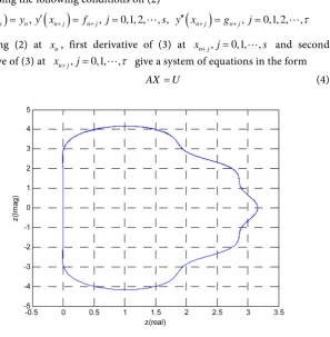
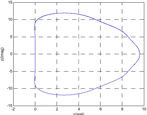
The aim of this paper is to develop a class of second derivative linear multistep method with varying step-lengths which are A-stable with large region of absolute stability (see Figures 1-3). The three methods recovered are tested on some numerical examples and their results compared with each other in order to determine how to fix the varying step-lengths to obtain the best results as shown
Tables 1-4.
2. Development of the Method
We considered the approximate solution of the form
( )
0 j
n n n
y x a x
=
=
∑
(2)where an’s are constants to be determined. The ith derivative of (2) gives ( )
( )
(
)(
) (
)
1 2
j
i n i
n n i
y x n n n n i a x −
−
=
∑
− − − (3)Imposing the following conditions on (2)
( )
n n,( )
n j n j, 0,1, 2, , ,( )
n j n j, 0,1, 2, ,y x =y y x′ + = f + j= s y′′ x+ =g+ j= τ
evaluating (2) at xn, first derivative of (3) at xn j+ ,j=0,1,,s and second
derivative of (3) at xn j+ ,j=0,1,,
τ
give a system of equations in the form [image:2.595.241.539.410.714.2]AX =U (4)
DOI: 10.4236/ajcm.2018.81008 98 American Journal of Computational Mathematics Figure 2. Showing RAS for Case 11.
Figure 3. Showing RAS for Case III.
where
(
)
(
)
(
)
2 3
2 1
2 1
1 1 1
2 1
2
2
1 1
2
1
0 1 2 3
0 1 2 3
0 1 2 3
0 0 2 6 1
0 0 2 6 1
0 0 2 6 1
j
n n n n
j
n n n
j
n n n
j
n s n s n s
j
n n
j
n n
j
n n
x x x x
x x jx
x x jx
X x x jx
x j j x
x j j x
x τ j j x τ
− −
+ + +
−
+ + +
− −
+ +
−
+ +
=
−
−
−
[
]
T[
]
T0 1 s 2 , n n n s n n
[image:3.595.248.499.309.505.2]DOI: 10.4236/ajcm.2018.81008 99 American Journal of Computational Mathematics Table 1. Showing Results of Example 1.
x h yi Case I Case II Case III
10 0.1 y1 4.28E−22 3.94E−19 2.13E−18
y2 4.49E−24 4.15E−21 2.24E−20
0.05 y1 1.65E−24 1.67E−21 9.23E−21
y2 1.29E−26 1.76E−23 9.72E−23
0.001 y1 4.96E−24 4.96E−24 4.14E−24
y2 5.17E−26 5.17E−26 4.52E−26
15 0.1 y1 2.89E−26 2.68E−23 1.45E−22
y2 3.03E−28 2.83E−25 1.53E−24
0.05 y1 2.27E−28 1.14E−25 6.29E−25
y2 2.37E−30 1.20E−27 6.62E−27
0.001 y1 4.04E−28 4.80E−28 3.53E−28
y2 4.34E−30 5.13E−30 3.94E−30
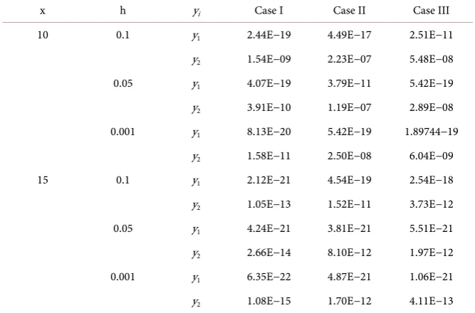
Table 2. Showing Results for Example 2.
x h yi Case I Case II Case III
10 0.1 y1 2.44E−19 4.49E−17 2.51E−11
y2 1.54E−09 2.23E−07 5.48E−08
0.05 y1 4.07E−19 3.79E−11 5.42E−19
y2 3.91E−10 1.19E−07 2.89E−08
0.001 y1 8.13E−20 5.42E−19 1.89744−19
y2 1.58E−11 2.50E−08 6.04E−09
15 0.1 y1 2.12E−21 4.54E−19 2.54E−18
y2 1.05E−13 1.52E−11 3.73E−12
0.05 y1 4.24E−21 3.81E−21 5.51E−21
y2 2.66E−14 8.10E−12 1.97E−12
0.001 y1 6.35E−22 4.87E−21 1.06E−21
y2 1.08E−15 1.70E−12 4.11E−13
Solving (4) using cramer’s method for the unknown constants, substitute it into (2), we obtain continuous linear multistep method in the form
( )
2( )
0 0
s
n t n j n j j n j
j j
y y h t f h t g
τ
β η
+ + +
= =
= +
∑
+∑
(5)subject to 0
( )
s j j
h
∑
=β
t =th, βj( )
t and ηj( )
t are polynomial of degree1
s+ +τ . Evaluating (5) at selected grid points give a block method in the form
( )1 ( )0
(
( )0 ( )1)
2(
( )0 ( )1)
1 1 1
m m m m m m
Y Y h F F h G G
ζ
+ =ζ
+η
+η
+ +γ
+γ
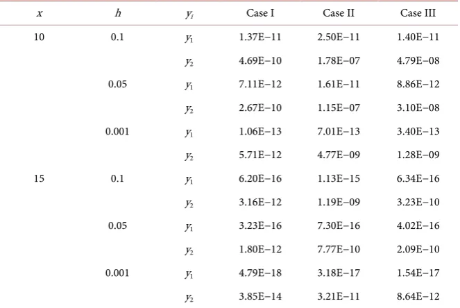
+ (6) [image:4.595.206.540.344.564.2]DOI: 10.4236/ajcm.2018.81008 100 American Journal of Computational Mathematics Table 3. Showing Results for Example 3.
x h yi Case I Case II Case III
10 0.1 y1 1.37E−11 2.50E−11 1.40E−11
y2 4.69E−10 1.78E−07 4.79E−08
0.05 y1 7.11E−12 1.61E−11 8.86E−12
y2 2.67E−10 1.15E−07 3.10E−08
0.001 y1 1.06E−13 7.01E−13 3.40E−13
y2 5.71E−12 4.77E−09 1.28E−09
15 0.1 y1 6.20E−16 1.13E−15 6.34E−16
y2 3.16E−12 1.19E−09 3.23E−10
0.05 y1 3.23E−16 7.30E−16 4.02E−16
y2 1.80E−12 7.77E−10 2.09E−10
0.001 y1 4.79E−18 3.18E−17 1.54E−17
[image:5.595.205.541.345.649.2]y2 3.85E−14 3.21E−11 8.64E−12
Table 4. Showing Results for Example 4.
x h yi Case I Case II Case III
15 0.1 y1 1.60E−09 2.27E−10 2.23E−10
y2 6.94E−18 6.94E−18 1.04E−17
y3 8.88E−16 8.88E−16 1.78E−15
y4 1.11E−16 1.11E−16 1.67E−16
0.05 y1 1.51E−09 2.28E−10 2.23E−10
y2 1.39E−17 1.04E−17 1.04E−17
8.88E−16 8.88E−16 8.88E−16 2.78E−17 8.33E−17 8.33E−17
0.001 y1 1.43E−09 2.48E−10 2.23E−10
y2 6.94E−18 3.47E−17 2.43E−17
8.88E−16 3.55E−15 2.22E−15 2.78E−17 1.94E−16 8.33E−17
[
]
T[
]
T1 1 2 , 1 2
m n n n s m n n n
Y + = y+ y+ y+ F = f − f − f
[
]
T[
]
T1 1 2 , 1 2
m n n n s m n n n
F + = f + f + f+ Y = y− y− y
[
]
T[
]
T1 2 , 1 1 2
m n n n m n n n
G = g− g− g G + = g+ g+ g+τ
Writing (6) in the form
(
)
( )0(
( )0 ( )1)
2(
( )0 ( )1)
1 1 1 1 0
m m m m m m m
F Y+ =Y + −
ζ
Y −hη
F +η
F + −hγ
G +γ
G + = (7)DOI: 10.4236/ajcm.2018.81008 101 American Journal of Computational Mathematics
( )
1( )
11 1 1
m m m
Yκ Yκ Jκ F Yκ
− +
+ = + − + (8)
where Jκ is the Jacobian matrix. The necessary and sufficient condition for
convergence of (8) is that the spectral radius of the inverse of the Jacobian
matrix
( )
11
Jκ
ρ
− <(
)
(
)
(
)
(
)
(
)
(
)
(
)
(
)
(
)
(
)
(
)
(
)
(
)
(
)
(
)
( )
(
)
1 2 1 1
1 1 1 1 1 1
1 2 1 2
2 2 2 2 2 2
2
2
n n n s n n n
n n n n n n
n n n s n n n
n n n n n n
n s n s n s n
n s n s n s n s n s
F y F y F y G y G y G y
y y y y y y
F y F y F y G y G y G y
J y y y y y y
F y F y F y G y G y
y y y y y
τ τ + + + + + + + + + + + + + + + + + + + + + + + + + + + + + + + + + ∂ ∂ ∂ ∂ ∂ ∂ ∂ ∂ ∂ ∂ ∂ ∂ ∂ ∂ ∂ ∂ ∂ ∂ = ∂ ∂ ∂ ∂ ∂ ∂ ∂ ∂ ∂ ∂ ∂ ∂ ∂ ∂ ∂ ∂
(
n)
n s G y y τ + + ∂ ∂
Specification of the Method
In this paper, we consider grid points xn j+ ,j= < < <0 u v w, hence the (6)
reduces to
( )1 ( )0 ( )0 11
21
31
1 0 0 0 0 1 0 0
0 1 0 , 0 0 1 , 0 0
0 0 1 0 0 1 0 0
θ
ζ ζ η θ
θ = = =
( )1 12 13 14 ( )0 15 ( )1 16 17 18
22 23 24 25 26 27 28
32 33 34 35 36 37 30
0 0
, 0 0 ,
0 0
θ θ θ θ θ θ θ
η θ θ θ γ θ γ θ θ θ
θ θ θ θ θ θ θ
= = =
[
]
T[
]
T1 , 1 2 ,
m n u n v n w m n n n
Y + = y+ y+ y+ Y = y− y− y
[
]
T[
]
T1 2 , 1 ,
m n n n m n u n v n w
F = f − f − f F + = f + f+ f +
[
]
T[
]
T1 2 , 1
m n n n m n u n v n w
G = g − g − g G + = g + g + g +
5 5 3 3 4 2 3 3 4 2 3 3 4
2 3 3 2 2 3 2 3 3 2 3 2
11 3 3
5 5 14 16 14 16 210 23
56 56 28 28 40 40
420
u v u w u v u v u w u w v w u vw
uv w uv w u vw u v w u vw u v w u v w θ + + − + − + − − − − − + + =
(
) (
)
5 5 3 3 4 2 3 3 4 2
3 3 6 2 2 2 4 2 3
3 2 2 3 2 3 3 2 3 2
12 3 3
350 350 140 388 140 388
210 105 1554 1187 574
574 490 490 1342 1342
420
u v u w u v u v u w u w
v w u u v w u vw uv w
uv w u vw u v w u vw u v w u
u w u v θ − − − + − + + + + + − − + + − − = − −
(
) (
)
4 4 2 3 3 2 2 3 3 2 2 3 3 2
3 3 3 2 2 2 2 2 2
5
13 3 3 3
10 5 28 35 14 16 70 98
70 98 10 42 46 98
420
u v u w u v u v u w u w v w v w
uvw uv w u vw uv w u vw u v w u
v v w u v θ − + − − + − + + − − − − + = − − −
(
) (
)
4 4 2 3 3 2 2 3 3 23 2 3 2
3 3 3 2 2 2 2 2 2
5
14 3 3 3
5 10 14 16 28 35 98 70
98 70 10 42 98 46
420
u v u w u v u v u w u w v w v w
uvw uv w u vw uv w u vw u v w u
DOI: 10.4236/ajcm.2018.81008 102 American Journal of Computational Mathematics
3 3 2 2 2 2 2 2
4 2 2 2
2
15 2 2
16 16 14 14 70
5 56 56 56
840
u v u w u v u w v w
u uvw uv w u vw u v w θ − − + + + + − − + =
(
) (
)
3 3 2 2 2 2 2 2
4 2 2 2
2
16 2 2
40 40 28 28 70
15 84 84 112
840
u v u w u v u w v w
u uvw uv w u vw u
u w u v θ − − + + + + − − + = − − −
(
) (
)
2 2 2 2 3
5
17 2 2 2
8 14 16 28 5 28
840
u v uw u w vw u uvw u
v v w u v
θ = − + − − + +
− −
(
) (
)
2 2 2 2 3
5
18 2 2 2
14 16 8 28 5 28
840
uv u v u w v w u uvw u
w v w u w
θ = − − − + +
− −
5 5 2 4 3 3 3 3 3 3
4 2 4 2 3 3 2 2 3
2 3 3 2 3 2
21 3 3
5 5 16 14 210 14
16 23 28 40 56
40 56 28
420
uv v w u v u v u w v w
v w uv w uv w uv w u vw
u v w u vw u v w v u w θ + − + + + − − − + − + − − =
(
) (
)
4 4 2 3 3 2 2 3 3 2 2 3 3 2
3 3 3 2 2 2 2 2 2
5
22 3 3 3
10 5 35 28 70 98 14 16
70 10 98 46 42 98
420
uv v w u v u v u w u w v w v w
uvw uv w u vw uv w u vw u v w v
u u w u v θ − − + − + − + + − − − − + = − −
(
) (
)
5 5 2 4 3 3 3 3 3 3
4 2 6 2 2 2 4 2 3
3 2 2 3 2 3 3 2 3 2
23 3 3
350 350 388 140 210 140
388 105 1554 1187 490
1342 574 1342 574 490
420
uv v w u v u v u w v w v w v u v w uv w uv w
uv w u vw u v w u vw u v w v
v w u v
θ + − + − + − − − − − + + + + − = − −
(
) (
)
4 4 2 3 3 2 2 3 3 2 2 3 3 2
3 3 3 2 2 2 2 2 2
5
24 3 3 3
5 10 16 14 98 70 28 35
98 10 70 98 42 46
420
uv v w u v u v u w u w v w v w
uvw uv w u vw uv w u vw u v w v
w v w u w θ − − + − + − + + + − − + + = − − −
3 3 2 2 2 2 2 2
4 2 2 2
2
25 2 2
16 16 14 70 14
5 56 56 56
840
uv v w u v u w v w
v uvw uv w u vw v u w θ − − + + + + − + − =
(
) (
)
2 2 2 2 3
5
26 2 2 2
8 28 14 16 5 28
840
uv uw vw v w v uvw v
u u w u v
θ = − + − + − −
− −
(
) (
)
3 3 2 2 2 2 2 2 4
2 2 2
2
27 2 2
40 40 28 70 28 15
84 112 84
840
uv v w u v u w v w v
uvw uv w u vw v
v w u v θ − − + + + + − + − = − − −
(
) (
)
2 2 2 2 3
5
28 2 2 2
16 14 28 8 5 28
840
uv u v u w v w v uvw v
w v w u w
θ = − + − − + +
DOI: 10.4236/ajcm.2018.81008 103 American Journal of Computational Mathematics
5 5 3 3 2 4 3 3 2 4 3 3 4
2 3 3 2 2 3 2 3 3 2 3 2
31 3 3
5 5 210 16 14 16 14 23
40 28 40 56 28 56
420
uw vw u v u w u w v w v w uvw
uv w uv w u vw u v w u vw u v w w u v θ + + − + − + − + − + − − − =
(
) (
)
4 4 2 3 3 2 2 3 3 2 2 3 3 2
3 3 3 2 2 2 2 2 2
5
32 3 3 3
10 5 70 98 35 28 16 14
10 70 98 46 98 42
420
uw vw u v u v u w u w v w v w
uvw uv w u vw uv w u vw u v w w
u u w u v θ − − + − + + − − + − − + − = − −
(
) (
)
4 4 2 3 3 2 2 3 3 2 2 3 3 2
3 3 3 2 2 2 2 2 2
5
33 3 3 3
5 10 98 70 16 14 35 28
10 98 70 98 46 42
420
uw vw u v u v u w u w v w v w
uvw uv w u vw uv w u vw u v w w
v v w u v θ − − + − + + − + + − − + + = − −
(
) (
)
5 5 3 3 2 4 3 3 2 4
3 3 6 2 2 2 4 2 3
3 2 2 3 2 3 3 2 3 2
34 3 3
350 350 210 388 140 388
140 105 1554 1187 1342
490 1342 574 490 574
420
uw vw u v u w u w v w v w w u v w uvw uv w
uv w u vw u v w u vw u v w w
v w u w
θ − − + + − + − + + + − + − − + − = − −
3 3 2 2 2 2 2 2
4 2 2 2
2
35 2 2
16 16 70 14 14
5 56 56 56
840
uw vw u v u w v w
w uvw uv w u vw w u v θ − − + + + + + − − =
(
) (
)
2 2 2 2 3
5
36 2 2 2
28 8 16 14 5 28
840
uv uw vw v w w uvw w
u u w u v
θ = − + + − − −
− −
(
) (
)
2 2 2 2 3
5
37 2 2 2
28 16 14 8 5 28
840
u v uw u w vw w uvw w
v v w u v
θ = − + − + − −
− −
(
) (
)
3 3 2 2 2 2 2 2
4 2 2 2
2
38 2 2
40 40 70 28 28
15 112 84 84
840
uw vw u v u w v w
w uvw uv w u vw w
v w u w θ − − + + + + + − − = − − −
For our methods, in case 1, we considered one step method with two hybrid
points with equal interval where 1, 2, 1
3 3
u= v= w= . For case II, we considered
two step method with one hybrid points with equal interval, where
1, 3 2, 2
u= v= w= and for the lase case III, we considered three step method
with equal interval where u=1,v=2,w=3.
3. Stability Properties
In this section, we investigate the basic properties of the developed method vis-a-vis order, local truncation error, consistency, zero-stability, convergence, and region of absolute stability of the methods.
3.1. Order of Convergence
DOI: 10.4236/ajcm.2018.81008 104 American Journal of Computational Mathematics
( )
( )1 ( )0(
( )0 ( )1)
2(
( )0 ( )1)
1 1 1
: m m m m m m
y x h =
ζ
Y + −ζ
Y −hη
F +η
F+ −hγ
G +γ
G +
(9)
where y x
( )
is an arbitrary function, continuously differentiable on an interval[
x xn, N]
. Ehigie, J. O. and Okunuga [11] can be written in Taylor expansion as( )
( )
( )
2( )
( )( )
0 1 2
: n n n q q q n
y x h =c y x +c hy' x +c h y′′ x + +c h y x +
where
(
)
11 1
1 1
1 !
r r
p p
p j j
j j
c j j
p θ p γ
−
= =
= −
−
∑
∑
(9) is of order p if
( )
( )
10 1 1
: p , p p 0
y x h =o h + c = =c =c ≠c+ =
1 p
c + is called the error constant and 1 1 ( 1)
( )
p p p
c+h +y + x is called the local
truncation error (LTE).
For our scheme, the order is 8 with error constant given by
(
)
(
)
9
5 3 3 2 2 2 2 2 2 4 2 2 2
9
5 3 3 2 2 2 2 2 2 4 2 2 2
9
5 3 3 2 2 2 2 2 2 4 2
15 15 12 12 42 5 42 42 48
50803200
15 15 12 42 12 5 42 48 42
50803200
15 15 42 12 12 5 48 42
50803200
h
u u v u w u v u w v w u uvw uv w u vw h
v uv v w u v u w v w v uvw uv w u vw h
w uw vw u v u w v w w uvw u
− − + + + + − − +
− − + + + + − + −
− − + + + + + −
(
2 2)
42
v w u vw
−
3.2. Consistency
Definition 1 A block method is consistent if it has order p≥1.
3.3. Zero-Stability
Definition 2 A method is said to be Zero-stable if no root of the first characteristics polynomial has modulus greater than one, and if every root of modulus one has multiplicity not greater than one or is simple.
( )
1 0 0 0 0 1
0 1 0 0 0 1
0 0 1 0 0 1
ρ λ λ
= −
The roots of the determinant gives λ =0, 0,1, hence the method is consistent.
3.4. Convergence
Definition 3 A method is said to be convergent if It is consistent and zero stable.
3.5. Region of Absolute Stability (RAS)
Definition 4 The Region of absolute stability (RAS) of a L M M is the set R = {z=λh: for z where the root of the stability polynomial are absolute less than
one}.
Substituting the test equation 2
,
DOI: 10.4236/ajcm.2018.81008 105 American Journal of Computational Mathematics
region of absolute stability for our new methods are shown below:
In determining the region of absolute stability, we consider three cases in this paper as described below:
Definition 5 A-Stability
A method is said to be A-stable if its region of absolute stability contains the whole of the complex left hand-half plane Re
( )
hλ
<0 . Alternatively, anumerical method is called A-Stable if the solution tend to zero as n→ ∞
when the method is applied with fixed h to any differential equation of the form
y y x
λ
∂ =
∂ , where λ is a complex constant with negative real part. Hence, for our
cases I, II, & III; The regions of absolute stabilities are given in Figures 1-3. We conclude that the three cases presented in this paper are A-stable.
4. Numerical Experiments
In this section we considered four examples to test the efficiency of the method. We compared the results of the cases in order to conclude on the best way to fix
u,v and w. The following notations are used to show the results
10 .
e υυ
ψψ −υυ ψψ= ∗ −
Example 1 We consider a system in the range 0≤ ≤x 20
( )
1 95 1
,
1 97 1
y′ =− y y x =
− −
with the exact solution
( )
296 29595e 48e
1
47 48e e
x x
x x
y x
− −
− −
−
=
−
The eigenvalues of the Jacobian matrix are λ1= −2,λ2= −96 with the
stiffness ratio 1:48. Source :Abdulimen [10].
Example 2 We consider a simple nonlinear stiff system
( )
( )
1 1 1
2
2 1 2 2
, 0 5
2 , 0 5
y y y y y y y
′ = − =
′ = − =
[
0, 20]
x∈ , with the exact solution
( )
(
)(
)
1
2
5 exp
5 exp 2 1_5
y x
y x x
−
=
−
The eigenvalues of the Jacobian matrix are λ1= −1,λ2= −2. Source: Yakubu
and Markus [9].
Example 3 In the this example we consider stiff nonlinear system of two dimensional Kaps problem with corresponding initial conditions
( )
( )
( ) ( )
( )
(
( )
( )
)
( )
( )
2
1 1 2 1
2 1 2 2
0 1
1002 1000
,
0 1
1
y x y x y x y
y x y x y x y x y
′
− +
= =
′ − +
DOI: 10.4236/ajcm.2018.81008 106 American Journal of Computational Mathematics
( )
( )
(
( )
)
1
2
exp 2
exp
y x x y x x
−
=
−
Source: Yakubu and Markus [9].
Example 4 We consider a four dimensional problems
( )
( )
( )
( )
( )
( )
( )
( )
( )
( )
( )
( )
( )
( )
( )
( )
( )
( )
4
1 1 2 3 4 1
2 2 3 4 2
3 3 4 3
4 4 4
0 1
10 100 10
0 1
1000 10 10
0 1
10
0 1
0.1
y x y x y x y x y x y y x y x y x y x y
y x y x y x y
y x y x y
′
− + − +
′ − + −
= = =
′ − +
′ −
Within the range 0≤ ≤x 20. The eigenvalues of the Jacobian matrix
1 0.1
λ
= − ,λ
2= −10, λ = −3 1000 andλ
4 = −10000. The exact solution isgiven as
( )
0.11
1000 10000
89990090 818090
e e
8999010009 89901009
998911 89071119179
e e
899010090 89990100090
x x
x x
y x − −
− −
= − +
+ +
( )
0.1 10002
9100 910 9989911
e e e
8991 8991 9989001
x x x
y x = − − − + −
( )
0.13
100 91
e e
9 9
x x
y x = − − −
( )
0.14 e
x
y x = −
Source: Ehigie, Okunuga, and Sofoluwe [11].
5. Conclusion
In this paper, we introduced three new second derivative linear multistep methods for the numerical solution of stiff initial value problems. Four numerical examples were considered, the results justified the proficiency of the second derivative method which is cheaper to implement since it does not require starting values and particularly the new methods show that lower step method gives better accuracy than higher step methods of the same order. We are able to achieve the aim of this paper which is to develop a class of second derivative linear multistep methods that are A-stable with large region of absolute stabilityas shown in Figures 1-3. The results from the high-order methods are very encourging (see Tables 1-4), therefore, we recommend further investigation of the second-derivative.
References
[1] Ezzeddine, A.K. and Hojjati, G. (2012) Third Derivative Multistep Methods for Stiff Systems. International Journal of Non-Linear Sciences, 14, 443-450.
[2] Enright, W.H. (1974) Second Derivative Multistep Methods for Stiff Differential Equations. SIAM J. Numerical Analysis, 11, 321-331.
https://doi.org/10.1137/0711029
DOI: 10.4236/ajcm.2018.81008 107 American Journal of Computational Mathematics Methods. Technical Reports No. 16183, Development of Computer Sciences Uni-versity of Toronto, Canada.
[4] Brown, T.I. (1977) Some Characteristics of Implicit Multistep Multi-Derivative In-tegration Formulas. SIAM J. Numer. Math., 34, 59-84.
[5] Cash, J.R. (1981) On the Exponential Fitting of Composite Multi-Derivative Linear Multi Step Method. SIAM J. Numer. Anal, 18, 808-812.
https://doi.org/10.1137/0718055
[6] Okunuga, S.A. (1997) Fourth Order Composite Two Step Method for Stiff Prob-lems. Int. J. Comput. Math., 2, 39-47.
[7] Abhulimen, C.E. and Okunuga, S.A. (2008) Exponentially Fitted Second Derivative Multistep Method for Stiff Initial Value Problems for ODEs. J. Eng.Sci. Appl., 5, 36-47.
[8] Ngwane, F.F. and Jator, S.N. (2012) Block Hybrid Second Derivative Method for Stiff Systems. International Journal of Pure and Applied Mathematics, 80, 543-559. [9] Yakubu, D.G. and Markus, S. (2016) The Efficiency of Efficiency of Second
Deriva-tive Multistep Methods for the Numerical Integration of Stiff Systems. Journal of the Nigeria Mathematics Society, 35, 107-127.
[10] Abdulimen, C.E. (2014) Exponentially Fitted Third Derivative Three Step Method for the Numerical Integration of Stiff IVP. Applied Mathematics and Computation, 243, 446-453.