Detection and Prediction of
Changepoints
Jamie-Leigh Chapman, M.Math.(Hons.) M.Res
Submitted for the degree of Doctor of Philosophy
at Lancaster University.
This thesis focuses upon the detection and prediction of changepoints in time series.
In particular, we develop a range of methods, both parametric and non-parametric, to
detect, predict, and forecast in the presence of changepoints. We consider a range of
data applications. These include economic, environmental and telematics data sets.
The first part of this thesis concentrates on forecasting. We propose two approaches
to incorporate changepoints into the forecasting process. Each of these approaches
are flexible. Additionally, we develop methodology to predict future changepoints in
a time series. In particular, we can predict changepoints at both future time points,
and changes near the end of the time series for which we do not yet have enough
observations to detect. This also includes a new approach to pre-whitening time
series that accounts for changes in the second order structure of the explanatory time
series.
The second part of this thesis is concerned with changepoint detection. We introduce
methodology for detecting changes in both the variance and the autocovariance of time
series. To do this we consider a local measure of the variance and the autocovariance
over time. The approach is non-parametric and resilient to the presence of outliers.
I would like to thank all the staff and students, past and present, of the STOR-i
centre for doctoral training for providing such a supportive and rewarding research
environment. I am most grateful to my two supervisors Idris Eckley and Rebecca
Killick, both of whom has supported, encouraged and guided me over the years. I
only hope we can continue working together in the future.
I am very grateful for the financial support provided by the EPSRC and the Office
for National Statistics, and the academic support received from the BigInsight centre
for research-based innovation.
Special thanks are to Catherine Ridout who inspired me to pursue Mathematics, from
which I found my way to Statistics. I am very lucky to have had both her and Rebecca
Killick as strong female role models. I hope that I am able to have such a positive
influence on others in the future.
Lastly, I would like to express my utmost gratitude to my parents, my husband Aaron
and my best friend Matthew for their support.
I declare that the work in this thesis has been done by myself and has not been
submitted elsewhere for the award of any other degree.
The word count of this thesis is approximately 47,000.
A version of Chapter 6 has been accepted for publication as Chapman, J-L., Eckley,
I.A, Killick, R. (2019),A nonparametric approach to detecting changes in variance in locally stationary time series, Environmetrics.
Jamie-Leigh Chapman
1 Introduction 1
2 Literature Review 3
2.1 Introduction . . . 3
2.2 Single Changepoint Detection . . . 5
2.3 Binary Segmentation . . . 6
2.4 Penalised Cost Functions . . . 9
2.4.1 Dynamic Programming . . . 10
2.4.2 Cost Function . . . 13
2.4.3 Penalty . . . 15
2.5 Other Approaches . . . 16
2.5.1 Genetic Algorithm . . . 16
2.5.2 Hidden Markov Models . . . 17
2.5.3 Bayesian Methods . . . 17
2.6 Changes in Second Order Structure . . . 19
3 Changepoint Identification to Improve Forecasts 21 3.1 Introduction . . . 21
3.2 Preprocessing . . . 23
3.2.1 The Model . . . 25
3.2.2 Forecasting . . . 26
3.3 Modelling . . . 27
3.3.1 Forecasting . . . 29
3.4 Simulation Study . . . 30
3.5 Application to the United Kingdom’s Gross Domestic Product . . . . 38
3.6 Discussion and Conclusion . . . 40
3.A Appendix . . . 40
4 Predicting Future Changepoints 42 4.1 Introduction . . . 42
4.2 Changepoint Prediction Methodology . . . 45
4.2.1 Estimating d and S . . . 46
4.2.2 Single Changepoint Case . . . 48
4.2.3 Multiple Changepoint Case . . . 51
4.3 Predicting Future changepoints . . . 52
4.4 Simulation Study . . . 54
4.5 Piecewise Pre-whitening . . . 61
4.5.1 Method . . . 62
4.5.2 Simulation Study . . . 63
4.6 Data Application . . . 69
4.7 Conclusions and Future Work . . . 73
4.A Appendix . . . 74
5 Wavelets 76 5.1 Wavelets . . . 77
5.1.1 Fourier Properties of the Scaling Function . . . 80
5.1.2 Deriving a Wavelet Function from a MRA . . . 82
5.1.3 The Discrete Wavelet Transform . . . 84
5.2 Locally Stationary Time Series . . . 88
5.2.1 Stationary Time Series . . . 88
5.2.2 Locally Stationary Wavelet (LSW) Processes . . . 89
5.3 Changepoint Detection using Locally Stationary Wavelet Models . . . 93
6 A Nonparametric Approach to Detecting Changes in Variance in Locally Stationary Time Series 98 6.1 Introduction . . . 98
6.2 A Nonparametric Approach to Detecting Changes in Variance . . . . 99
6.2.1 Locally Stationary Wavelet Framework . . . 99
6.2.2 The NPLE Method . . . 102
6.2.3 Penalty Choice . . . 105
6.3 Simulation Study . . . 107
6.3.1 Random Outliers . . . 107
6.3.2 Fixed Outliers . . . 109
6.3.3 Heavy Tail Structure . . . 111
6.4 Application to Wind Speed Characterization . . . 112
6.5 Conclusion . . . 115
7 A Nonparametric Approach to Detecting Changes in Autocovariance in Locally Stationary Time Series 116 7.1 Introduction . . . 116
7.2 A Nonparametric Approach to Detecting Changes in Autocovariance 118 7.2.1 The Non-parametric Model . . . 119
7.3 Simulation Study . . . 121
7.4 Application to Telematics Data . . . 130
7.5 Conclusion . . . 132
A Local Autocovariance Estimation 137 A.1 The Curtailed Local Autocovariance Function . . . 138
A.2 Extension to Locally Stationary Processes and Other Wavelet Families 141
A.3 Correcting the Local Autocovariance Function . . . 148
A.4 Conclusion . . . 149
2.1 A change in (a) variance and (b) mean. . . 4
3.1 United Kingdom’s Gross Domestic Product quarter on quarter growth 22 3.2 A change in mean with its ACF. . . 24
3.3 Residuals for Yt with and without a regressor. . . 24
3.4 ROC curve for i.i.d and correlated data for a change in mean. . . 26
3.5 A realisation Yt from scenario (a) with detected changes in mean. . . 34
3.6 Rolling forecast for GDP data. . . 39
4.1 United Kingdom’s Gross Domestic Product quarter on quarter growth. 42 4.2 Wind speed in a region. . . 43
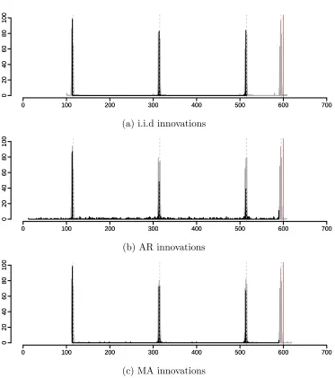
4.3 The response time series yt for the three changepoint cases. . . 48
4.4 Cross-correlation patterns for the three changepoint cases. . . 49
4.5 A realisation of the impulse time series xt. . . 54
4.6 Case 1, Case 2, and Case 3. . . 56
4.7 Results for Case 1. . . 57
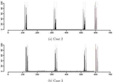
4.8 Results for Case 2 and 3. . . 60
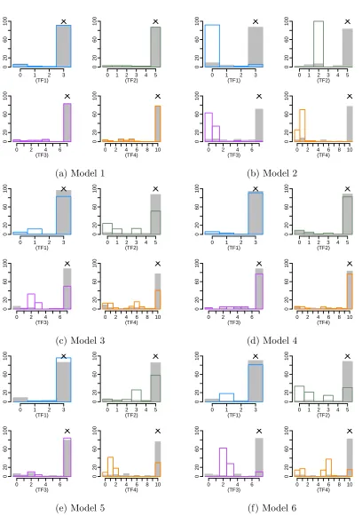
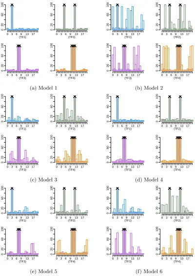
4.9 Delay results for models (1) - (6) and (a) - (d). . . 67
4.10 Set S results for models (1) - (6) and (a) - (d). . . 68
4.11 Speed over time of two HGVs. . . 70
4.12 Predicted changepoints for N = 100. . . 71
4.13 Predicted changepoints for n = 115. . . 72
4.14 Predicted changepoints for n = 150. . . 73
5.1 Examples of Daubechies extremal phase mother wavelets. . . 78
5.2 Haar Multi-resolution Analysis. . . 81
5.3 Wavelet transforms using the Haar wavelet. . . 86
6.1 Local smoothed and unsmoothed variance function. . . 101
6.2 Example plot of the number of changepoints against the cost function for a model with two changes in variance. From the plot we can cor-rectly identify the true number of changes to be two. . . 105
6.3 Density of detected changepoint locations. . . 108
6.4 Outliers model with detected changes in variance. . . 110
6.5 Detected changepoint locations for the Generalised Extreme Value data.112 6.6 Wind speed data. . . 113
6.7 Diagnostics plots. . . 114
6.8 Changepoint plots for NPLE and MLvar. . . 114
7.1 Smoothed and unsmooth local autocovariance function. . . 118
7.2 The local autocovariance function for Model E. . . 125
7.3 Detected changes in autocovariance. . . 127
7.4 Detected changes in autocovariance with outliers. . . 129
7.5 Acceleration data for a car journey. . . 130
7.6 Mapped changepoint locations for the accelaration data. . . 131
A.1 Leakage in the local autocovariance function using the Haar wavelet. 143 A.2 The local autocovariance function for HaarMA(2) and MA(3). . . 145
A.3 The bias in the local autovariance as N increases. . . 147
3.1 Results for in-sample forecasts for Models (A)-(G). . . 32
3.2 Results for out-of-sample forecasts for Models (A)-(G). . . 33
6.1 Proportion of changepoints detected for different percentages of outliers.108 6.2 Proportion of changepoints detected for the outliers model. . . 110
6.3 Proportion of changepoints detected for the simulated GEV data. . . 111
7.1 Results for scenario (A). . . 122
7.2 Results for scenarios (B)-(D). . . 123
7.3 Results for scenarios (E)-(G). . . 123
7.4 Results for scenarios (B)-(D) when subjected to 1% outliers. . . 128
7.5 Results for scenarios (E)-(G) when subjected to 1% outliers. . . 128
Introduction
Data is becoming increasingly important to industries operationally and, with an
up-rise in the number of companies that provide data warehousing and other cloud based
data management services, it is becoming faster and cheaper to perform large scale
analytics. Consequently, time series are increasing in size.
Forecasting is one of the many important areas of time series analysis. When
fore-casting it is often assumed that the statistical properties of the time series remain
constant throughout time. However, as a time series becomes longer, this assumption
is less likely to hold. The focus of this thesis is the development of methods to detect
such changes and incorporate them into forecasting.
Chapter 2 provides a literature review of changepoint detection with a focus upon
time series. Throughout this review, it is apparent that change detection is of use
in a multitude of application areas. This is reflected within this thesis. Chapter 3
considers microeconomic data, whereas Chapters 4 and 7 focus upon Telematics data.
In contrast, Chapter 6 has an environmental focus.
Chapter 3 builds upon the changepoint methodology, reviewed in Chapter 2, to
pro-pose two methods for using changepoints to improve forecasts. The first considers
identifying changes during the data preprocessing stage before building our
forecast-ing model. The second detects changes in the model we use to forecast the time series.
This chapter allows forecasts to be produced in the presence of changepoints however,
it does not have the facility to forecast changes explicitly. Hence, Chapter 4 introduces
a framework in which future changepoints can be predicted. This methodology relies
on constructing a relationship between two time series which both exhibit related
changes. The location of changes in one series are then used to estimate the changes
in the other. Chapter 4 also introduces an alternative approach to pre-whitening
time series, which does not rely on the assumption of second order stationarity. This
methodology exploits the changepoint detection methodology introduced in Chapter
3.
Chapters 3 and 4 highlight that many aspects of time series modelling rely on
ef-fectively capturing second order dependence structure. The methodology in Chapter
3 has the ability to capture changes in the second order structure of a time series,
however it is limited to assuming that the time series follows an autoregressive (AR)
or a moving average (MA) model. The remainder of this thesis seeks to remove this
AR/MA assumption. These chapters use wavelets in their approach. Wavelets are
suited to modelling the time-varying second order structure of time series due to
their localisation properties. Chapter 5 provides a review of wavelets and outlines the
methodology required as a basis for Chapters 6 and 7. Chapter 6 introduces a method
to detect changes in the variance of a time series and Chapter 7 generalises this to the
case of the autocovariance. These methods make no AR/MA assumptions on model
form. It is demonstrated that each of these methods are robust to the presence of
Literature Review
In this literature review we focus upon changepoint analysis. This provides a basis
for the first part of this thesis. In Chapter 5, we provide a separate literature review
on wavelets.
2.1
Introduction
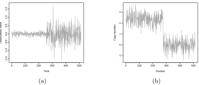
Achangepoint is a point, or position, in an ordered data sequence where the statistical properties change in some way. For example a changepoint could represent a point
in time such that the variance of the observations prior to the change differ to those
after the change, see for example Figure 2.1a. Alternatively for genomic data, in
which observations are ordered by position on a chromosome, a changepoint could
indicate a position where the mean level of the copy number of the DNA is smaller
prior to the change, than afterwards, see for example Figure 2.1b.
Specifically in a time series setting, changepoints could occur in lower order
struc-tures, such as the mean, or they could occur in higher order structures such as the
autocovariance. More than one statistical property could change at the same time. It
Time
Obser
v
ation V
alue
0 100 200 300 400 500
−1.5
−1.0
−0.5
0.0
0.5
1.0
1.5
(a)
0 100 200 300 400 500
−1
0
1
2
3
Position
Cop
y Number
[image:15.612.151.498.72.220.2](b)
Figure 2.1: Two examples of changepoints: (a) a point in time where the variance changes and (b) a position along a chromosome where the mean level changes.
is vital, in a modelling or forecasting setting, that we account for changepoints within
our frameworks, failure to do so will result in flawed inference. As a consequence of
the practical importance of changepoints, a vast literature surrounding the area has
arisen over the last fifty years.
Since the early work in changepoints by Page (1954) in the context of quality control,
changepoint detection methods have been extensively developed in a range of different
application areas. Some classical applications of changepoint detection include:
cli-matology (Reeves et al., 2007; Ruggieri et al., 2009); finance (Spokoiny, 2009; Andreou
and Ghysels, 2009); model validation (Fryzlewicz and Subba Rao, 2010). More
mod-ern applications include network security (Lvy-Leduc and Roueff, 2009; Bodenham
and Adams, 2014), neuroscience (Aston et al., 2012; Kirch et al., 2015) and linguistics
(Kulkarni et al., 2015).
In this chapter we discuss a range of approaches to the problem of detecting
points. We restrict our attention to the problem of retrospectively detecting
change-points in an “off-line” setting. The contrasting sequential setting is described by Lai
(1995) and Polunchenko and Tartakovsky (2012). For a general review of changepoint
detection we refer the reader to (Carlstein et al., 1994; Chen and Gupta, 2013; Eckley
The aim of this chapter is to form the basis for the work presented in Chapters 3
and 4 of this thesis. To begin, in Section 2.2 we introduce the single changepoint
model. Then in Section 2.3 we introduce binary segmentation and its variants. These
can be used to extend any single changepoint model into the multiple changepoint
setting. In Section 2.4 we describe the penalised cost function approach to multiple
changepoint detection and in Section 2.5 we briefly review some other changepoint
frameworks. Specifically, in Section 2.6 we review changepoint detection methods
focused on second order structure.
2.2
Single Changepoint Detection
Consider an ordered data sequence of length n, say y1:n = (y1, . . . , yn), and let Y1:n
be the corresponding sequence of random variables. Then, following the notation
of Eckley et al. (2011), a single changepoint occurs if there exists a location τ ∈ {1, . . . , n−1} such that the statistical properties of {y1, . . . , yτ} and {yτ+1, . . . , yn}
differ. It is natural to introduce the detection of a single changepoint as a
likelihood-ratio test.
The likelihood approach to detect changepoints was first proposed by Hinkley (1970)
for detecting changes in mean within a sequence of i.i.d. Normally distributed
obser-vations. This was later generalised to other distributions, for example Gamma (Hsu,
1979), Exponential (Haccou and Meelis, 1988), and Binomial (Hinkley and Hinkley,
1970). It has also been extended to detect changes in other properties of the data,
for example the variance (Chen and Gupta, 1997).
hypothesis test with the null and alternative hypothesis given by
H0 : No changepoint. H1 : A single changepoint.
Under the null hypothesis, H0, the maximum log-likelihood is given by`(y1:n|θˆ), where
`(·) is the log-likelihood of the probability density function associated with the entire
data and ˆθ is the maximum likelihood estimator of the parameters.
Assuming independence across segments, under the alternative hypothesis, the
max-imum profile log-likelihood for a given changepointτ ∈ {1,2, . . . , n−1}is given by
P r`(τ) =`(y1:τ|θˆ1) +`(yτ+1:n|θˆ2),
where ˆθi, i = 1,2, are the maximum likelihood estimators of the parameters for
segment i. The location of the changepoint is discrete, therefore the maximum
log-likelihood under H1 is: maxτP r`(τ).
The log of the likelihood ratio test statistic is:
λ(y1:n) = 2
h
max
τ P r`(τ)−`(y1:n|
ˆ
θ)i.
We then choose a thresholdβsuch that ifλ(y1:n)> β, we reject the null hypothesis. In
this case the position of the changepoint, ˆτ, is estimated by the profile log-likelihood
forτ:
ˆ
τ = arg max
τ P r`(τ).
In order to select the appropriate threshold β for a required significance level, the
asymptotic distribution for the likelihood ratio test must be attained. These
distribu-tions, and consequently the thresholds, for the case of Normal, Binomial and Poisson
In the following section, we illustrate how the likelihood approach could be extended
into a multiple changepoint setting.
2.3
Binary Segmentation
Binary segmentation (BS), first introduced by Scott and Knott (1974), is arguably
the most widely used method for detecting multiple changepoints and can be used
to extend any single changepoint method, for example the likelihood-ratio approach
(Eckley et al., 2011).
To perform binary segmentation we first apply the chosen single changepoint detection
method to the entire data set. If no changepoint is found then the algorithm has
finished. If a changepoint is detected, call this τ, then the data is split into two
segments, y1:τ and yτ+1:n. We then apply the single changepoint method to the two
segments and repeat iteratively. We stop when no further changepoints are detected.
Binary segmentation has since been implemented by Venkatraman (1992) and Chen
and Gupta (1997) to detect changes in independent Normal observations. Cho and
Fryzlewicz (2012) and Killick et al. (2013) have used it in conjunction with the wavelet
spectrum to detect changes in the second order structure of time series. Venkatraman
(1992) and Cho and Fryzlewicz (2012) prove the consistency of the algorithm in the
case of an unknown number of changepoints with additive and multiplicative errors,
respectively.
Despite being fast, O(nlogn), binary segmentation does have some disadvantages. A drawback to its computational efficiency is that it is only approximate. This is
because the changepoint locations identified are conditional on previously identified
changepoints. Another drawback is that binary segmentation may fail to identify
changepoints and the first and last segment follow the same distribution.
To overcome these drawbacks, Olshen et al. (2004) introduce a modification of BS,
called circular binary segmentation (CBS). At each iteration, this algorithm can detect
either a single changepoint or two changepoints. As the name suggests, it considers
the data in a circular fashion, and at each iteration the data within which you are
searching for a changepoint/s is joined at either end to form a circle.
Willenbrock and Fridlyand (2005) and Lai et al. (2005) both compare circular binary
segmentation against other methods for detecting changepoints in comparative
ge-nomic hybridization (CGH) data and show that it performs well, however from the
methods compared, Lai et al. (2005) conclude that CBS is one of the slowest. The
loss in computationally efficiency of circular binary segmentation is attributed to the
non-parametric methods used to calculate the p-value, and as such, the algorithm
grows quadratically with the length of the data.
A faster CBS algorithm is later developed by Venkatraman and Olshen (2007) in
which the p-value of the test statistic is calculated using a Gaussian random field.
A stopping rule is also added which limits the number of iterations of the algorithm
when there is strong evidence of a change. The changes implemented by Venkatraman
and Olshen (2007) improve the efficiency of CBS with only a small loss in accuracy.
Another modification to binary segmentation (BS) is wild binary segmentation (WBS)
(Fryzlewicz et al., 2014). This calculates the test statistic on random draws from the
data thereby sacrificing computation time for an increase in accuracy. This
modi-fication also alleviates the small segment issue and can identify changes of smaller
magnitude.
More specifically, WBS calculates the test statistic on multiple intervals with start
the test statistics are weighted according to the length of the interval and the largest
test statistic is tested against the threshold value.
In the WBS setting, in addition to choosing a threshold for detecting a changepoint,
the number of intervals drawn at each iteration also needs to be chosen. This
in-troduces a trade off between accuracy and computationally efficiency. An increased
number of intervals will increase accuracy, but this comes at a loss of computational
efficiency. Fryzlewicz et al. (2014) discuss the choice of penalty and number of
inter-val in order to obtain good results. In addition to having more tuning parameters,
WBS has increased computational time over BS, because the test statistic needs to
be computed for multiple intervals.
In summary, BS is easy to understand and it can be used with any changepoint test
thus providing a simple route from single changepoint detection to multiple changes.
However, there are clear disadvantages in terms of approximation error, which are
not wholly overcome by the new variants. The following section discusses a penalised
cost function approach to changepoint detection which, in contrast to BS, can be
guaranteed to give the optimal solution.
2.4
Penalised Cost Functions
In a multiple changepoint setting, one commonly used method is the penalised cost
function approach. Following Eckley et al. (2011), consider m changepoints with
positionsτ = (τ1, . . . , τm). Each changepoint position τi, is an integer between 1 and
n−1 and we define: τ0 = 0 and τm+1 =n. The changepoints are ordered such that:
τi < τj ⇐⇒ i < j. Thus themchangepoints split the data series intom+1 segments
with theith segment containingy
(τi−1+1):τi. In practice we impose a minimum segment
the changepoints, we aim to solve thepenalised minimisation problem:
min
m,τ1:m
m+1 X
i=1
C(y(τi−1+1):τi)
+βf(m), (2.1)
where C is a cost function over a segment and βf(m) is a penalty based on the number of changepoints m (Killick et al., 2012). The penalty term is introduced to
prevent over-fitting. An example penalty is the Schwarz Information Criterion (SIC,
(Schwarz et al., 1978)) (β =plogn), where pis the number of additional parameters
introduced by an additional changepoint. If this penalty is set too high, we run the risk
of under-fitting. Generally, the value of the threshold can have substantial impact on
the number of changepoints estimated, see Haynes et al. (2017a) for examples. The
function f(m) is often taken to be the number of changepoints m, resulting in a
penalty that is linear in the number of changepoints.
Detecting multiple changepoints is more computationally challenging than the single
changepoint case. Specifically, as the length of the data sequence increases, the
num-ber of possible changepoint positions increases rapidly. For this reason, much of the
multiple changepoint literature is dedicated to developing efficient algorithms.
In the following, in Section 2.4.1, we first review dynamic programming approaches
to solving the minimisation problem in equation (2.4). In Section 2.4.2 we discuss
the choice of cost function in equation (2.4). Finally, in Section 2.4.3 we discuss the
choice of penalty for equation (2.4).
2.4.1
Dynamic Programming
The first dynamic programming approach to changepoint detection was undertaken by
Auger and Lawrence (1989) in their Segment Neighbourhood Search (SNS) algorithm.
number of changes 1, . . . , M it determines the best partition of the data. This solves
a constrained version of equation (2.4). The computation is of orderO(M n2). This method does not have a choice of penalty but as, in practice, the number of changes
is often unknown, it can be equally difficult to return a single segmentation.
Jackson et al. (2005) introduce Optimal Partitioning (OP) which improves upon
Seg-ment Neighbourhood Search. Optimal Partitioning requires no such assumption on
the number of changes in the data and is instead of order O(n2). It aims to solve the penalised minimisation problem in equation (2.4). In contrast to creating a
dy-namic program across the number of changes, Jackson et al. (2005) create a dydy-namic
program across time. This requires no upper bound on the number of changes but a
penalty must be chosen.
Exploring the structure of this dynamic program further, OP first conditions on the
last point of change and then calculates the optimal segmentation of the data up
until that point. As the segments are independent, if we know the position of the last
changepoint, then we can use this to calculate those prior to it. Thus if for every time
point we know when the last change was prior to that, we can reconstruct the entire
segmentation.
Formally, let F(n) be a minimisation from equation (2.4) with f(m) = m. Then we
can write
F(n) = min
τ
(m+1
X
i=1
C(y(τi−1+1):τi)+β
)
.
Then, denote the last changepoint τm as τ∗. If we condition on the location of the
last change, then we can obtain
F(n) = min
τ∗
(
min
τ|τ∗ m
X
i=1
C(y(τi−1+1):τi)) +β
+C(y(τ∗+1):n) +β
)
. (2.2)
iterative nature of this procedure, we can re-write equation (2.4.1) as
F(n) = min
τ∗
F(τ∗) +C(y(τ∗+1):n) +β .
Optimal Partitioning is of orderO(n2), so in order to make this approach faster, Killick et al. (2012) introduces the Pruned Exact Linear Time (PELT) algorithm. PELT is
based on the Optimal Partitioning method of Jackson et al. (2005), but involves
an inequality based pruning step within the dynamic program. PELT reduces the
computational cost of OP whilst maintaining the exactness of the method.
PELT considers the data sequentially and the optimal segmentation up to that time
point. At each time point, Killick et al. (2012) demonstrate that the number of
changepoint configurations is restricted. For all times t < s < n, it is assumed there
exists a constant K such that,
C(y(t+1):s) +C(y(s+1):n) +K ≤ C(y(t+1):n).
Then, defining F(·) as in equation (2.4.1), if
F(t) +C(y(t+1):s) +K ≥F(s)
holds, at a future timen > s, t can never be the optimal last changepoint prior ton.
This means that timet does not need to be considered in the calculations for future
times greater thann for the rest of the dynamic program. Most cost functions satisfy
this condition and Killick et al. (2012) provide details on the selection ofK. If the cost
function is the negative log-likelihood, then K = 0. However, in order to obtain the
bound K, it must be assumed that the number of changepoints in the data increases
or pruning step, means that the number of changepoint configurations is bounded by
a constant number, K, at each time step. Thus PELT is of order O(Kn). In the case that the number of changepoint does not increase linearly with the length of the
data, PELT can not achieve O(Kn), and so PELT is best in applications where the number of changepoints is large.
Maidstone et al. (2017) introduce a similar method to PELT which also uses inequality
based pruning, but instead they apply it to SNS and call it Segment Neighbourhood
with Inequality Pruning (SNIP), however this performs poorly in comparison to
prun-ing SNS usprun-ingfunctional pruning.
Rigaill (2015) introduce an algorithm called pDPA, and this is a pruned version of
Segment Neighbourhood Search (Auger and Lawrence, 1989). Instead of performing
inequality based pruning, they use functional pruning. Rigaill (2015) show empirically
that the time complexity of pDPA isO(Knlogn). A drawback of pDPA is that it is necessary to calculate and store the values of multiple cost functions. Additionally,
as it implements functional pruning, it can only be used to detect changes in a single
parameter.
Similarly, Maidstone et al. (2017) introduce Functional Pruning Optimal Partitioning
(FPOP) which uses functional pruning on OP and they show that this always prunes
more than PELT. They also perform an empirical study which suggests that FPOP is
computationally efficient for large datasets regardless of the number of changepoints.
However, once again, as this implements functional pruning, it can only be used to
2.4.2
Cost Function
Cost functions for changepoint detection can be categorised as those which are
para-metric and based upon the likelihood of the data, and those which are non-parapara-metric
and so make no assumptions on the distributional form of the data.
When using the likelihood as the basis for a cost function of a segment, we use a scaled
maximum log-likelihood: −log`(y(τi−1+1):τi|θˆ), where θ is the vector of parameters in
which we want to find changes in. For example, changes in mean in i.i.d. Gaussian
data can be detected by replacing the cost function C(·) in equation (2.4) with twice the negative log-likelihood for a Gaussian distribution with common variance and
segment specific mean. For the data in a segment y(τi−1+1):τi, the segment cost of
twice the negative log-likelihood will be
C(y(τi−1+1):τi) =
1
σ2
τi
X
j=τi−1+1
(yj−µˆ)2,
where ˆµ is the maximum likelihood estimator for the segment mean.
A likelihood based cost function is effective if the distributional assumptions are
realis-tic. However, as the data becomes increasingly different from the chosen distribution,
the power to detect a changepoint will decrease. Therefore, if we model the data
using the wrong distribution, changepoint locations are less reliable. Consequently, a
non-parametric cost function may be preferable.
A commonly used non-parametric cost function for a segment is the quadratic loss
function, defined as
τi
X
t=τi−1+1
(yt−θi)2 (2.3)
whereθiis the mean of the segment containing datayτi−1+1:τi. The use of the quadratic
loss function (2.4.2) approach is susceptible to outliers and Fearnhead and Rigaill
(2018) suggest the use of a cost function that increases at a slower rate in |y−θ|, these include the Huber loss and the biweight loss (Huber, 2011).
Alternatively, Zou et al. (2007) introduce a non-parametric equivalent to the scaled
log-likelihood. They propose a non-parametric log-likelihood function based upon the
empirical cumulative distribution function (CDF) and use this in a likelihood ratio
test to detect a single changepoint. This is later extended by Zou et al. (2014) into the
multiple changepoint setting using Segment Neighbourhood Search (SNS). Zou et al.
(2014)’s approach performs well however it is computationally slow,O(mn2+n3). This complexity is attributed to the pre-computation of the segment costs and running the
SNS algorithm.
Later, Haynes et al. (2017b) build upon Zou et al. (2014)’s approach in order to
improve the computationally efficiency; they simplify the segment cost using an
ap-proximation and use PELT instead of SNS. The resulting algorithm, which they call
ED-PELT, runs with expected computational cost ofO(n+n2logn).
Other approaches which use a non-parametric cost function include the “E-Divisive”
method of Matteson and James (2014). This uses a cost function which aims to
maximise a Euclidean distance between two sub-segments at each iteration of BS. It
is later used within a dynamic programming setting (James and Matteson, 2015).
Non-parametric approaches to changepoint detection can often be more robust as no
distributional assumptions are made, however if the distribution is known, a
para-metric approach will be more powerful.
Having discussed the choice of cost function for use in equation (2.4), we now turn
our attention to dynamic programming, an algorithm which can be used to solve this
2.4.3
Penalty
In a penalized cost setting, the final model determined will be dependent upon the
penalty used in equation (2.4). This penalty, consists of two components. The first,
is the constant β and the second is the function f(m). Usually, we set f(m) = m
such that it is linear in the number of changepoints (Killick et al., 2012). Picard et al.
(2005) and Birg´e and Massart (2007) offer some discussion on alternative penalty
choices. Choices for the constant β are more varied in the literature.
Examples of penalties which are commonly used include Akaike’s information criterion
(AIC, (Akaike, 1974)), Schwarz information criterion (SIC, (Schwarz et al., 1978)) and
the Hannan-Quinn information criterion (Hannan and Quinn, 1979), defined as
AIC : β = 2p
SIC : β =plogn
Hannan-Quin : β = 2plog logn,
respectively. Asymptotically, the SIC and the Hannan-Quin penalties result the
cor-rect number of changepoints, see Yao et al. (1988) for details. Despite this, the
Hannan-Quin penalty is less popular. The AIC is still popular despite it
asymptot-ically over estimating the number of changepoints (Birg´e and Massart, 2001). This
has also been observed in practice by authors such as Haynes et al. (2017a), Kim et al.
(2009) and Lavielle (2005). Alternatively, Lavielle (2005) propose an adaptive choice
of penalty.
In many applications it may not be appropriate to choose only one penalty and
seg-mentation. It may be better to have multiple segmentations of the data and then
choose the most suitable according to a practitioner or the task at hand.
that ensure these penalties provide consistent estimates may not be valid. For this
reason, more recently, Haynes et al. (2017a) propose a method “Changepoints for
a Range Of Penalties” (CROPS) which returns all possible segmentations for some
penalty range in a computationally efficient manner.
In the following, we now turn our attention to an alternative approaches to detecting
multiple changepoints.
2.5
Other Approaches
In Section 2.3 and 2.4 we described two approaches to detecting multiple changepoints.
Here we briefly review some alternative approaches to the problem. Specifically, in
Section 2.5.1 we describe a genetic algorithm approach, in Section 2.5.2 we describe
a hidden Markov model approach and finally in Section 2.5.3 we describe a Bayesian
approach to changepoint detection.
2.5.1
Genetic Algorithm
A genetic algorithm is like natural selection taking place in species evolution. Suppose
we have a set of solutions which have weights according to some optimization criterion,
then according to these weights, we select two ‘parent’ solutions. These two solutions
form a new ‘child’ solution whose genes consist of the best genes from the parents.
The procedure allows mutation to take place such that the algorithm does not get
stuck in local optima.
The use of a genetic algorithm for changepoint detection has been implemented by a
selection of authors. For example, Liang and Wong (2000) develop an evolutionary
(2006) use a genetic algorithm to detect changes in autocovariance in a time series
and Li and Lund (2012) follow by example to detect changes in the mean of climatic
time series.
The genetic algorithm approach has the advantage that it will produce high quality
segmentations very quickly. However the search is approximate and repeated runs on
the same data may not produce the same results.
2.5.2
Hidden Markov Models
Hidden Markov models (HMMs) are an extension of Markov models first developed
by Baum and Eagon (1967) at the Institute for Defense Analyses. They are used in
applications such as pattern recognition (Rabiner, 1989) and clustering (Knab et al.,
2003). A HMM can be characterised by an underlying process generating an
observ-able sequence. This latent process is a Markov process and generates observations.
Luong et al. (2012) provide an introduction the use of HMMs for changepoint analysis.
A HMM can be fitted using either a classical frequentist or a Bayesian framework
and the hidden states (segmentations) can be inferred using, for example, Viterbi
(Viterbi, 1967) and Posterior Decoding (Juang and Rabiner, 1991) algorithms, or
the Forwards-Backward equations (Baum et al., 1970). For a recent contribution to
changepoint detection using HMMs, please see the work of Ko et al. (2015), who
propose an extension to the HMM of Chib (1998).
2.5.3
Bayesian Methods
A Bayesian framework for changepoint analysis was first introduced by Chernoff and
Zacks (1964) for detecting a change in the mean of a sequence of independent normal
changepoints, the location of changepoints and also upon the parameters for each
segment. There are two ways to do this. The first is to put a prior on the number of
changepoints and then another prior for their position given the number of
change-points (Barry and Hartigan, 1992). The second formulation is to specify a prior for
both the number of changepoints and their positions indirectly through a distribution
for the length of each segment (Pievatolo and Green, 1998).
In the first case, if the number of changepoints is known, then Markov Chain Monte
Carlo (MCMC) is often used to estimate the changepoint locations and the
asso-ciated segment parameters (Stephens, 1994; Chib, 1996, 1998). When the number
of changepoints is unknown, a common approach is reversible jump MCMC (Green,
1995). Alternatively, Lavielle and Lebarbier (2001) propose a hybrid approach using
the Metropolis-Hastings algorithms with a Gibbs-sampler.
More recently, Schwaller and Robin (2017) extend the product partition model of
Barry and Hartigan (1992) by adding a graphical structure which could capture the
dependencies between multivariate observations.
In the second case, where a prior is placed on the duration of each segment, the
posterior can be sampled directly (Barry and Hartigan, 1993). This approach has
been taken by Liu and Lawrence (1999) for DNA sequencing and has been used
more generally by Fearnhead (2005) and Fearnhead (2006). This approach assumes
independence across segments. Consequently, Fearnhead and Liu (2011) extend their
approach to include dependence across segments.
More recent contributions include the work of Rigaill et al. (2012). They derive the
exact posterior distribution of changepoint locations for exponential random variables
with conjugate priors. This approach is later adapted by Cleynen and Robin (2016)
in order to compare multiple series. Most recently Hinoveanu et al. (2019) propose a
We refer the reader to Eckley et al. (2011) for a detailed outline of the Bayesian
changepoint framework and additional references can be found in Section 4.1.
2.6
Changes in Second Order Structure
Having focussed on changes in i.i.d. data sequences in the previous sections, in this
section we consider a different setting. Specifically, we review the literature on
detect-ing changes in the second order structure of a time series. We review contributions
made using the following three approaches: a classical likelihood approach, an
ap-proximate likelihood approach and finally a nonparametric approach. Davis et al.
(2006), Gombay (2008), Killick et al. (2013) and Fryzlewicz and Subba Rao (2014)
all take a likelihood approach to detecting changes in second order structure. Below
we briefly summarise each of these contributions.
The Auto-PARM approach of Davis et al. (2006) calculates the likelihood-based
mini-mum description length (MDL) (Jorma, 1998) of an autoregressive process of orderp.
The basic idea of MDL is that the best-fitting model is the one than enables maximum
compression of the data. The best fitting model, as decided by the MDL, is
deter-mined by optimizing some criterion. Davis et al. (2006) use a genetic algorithm to
explore the search space of this optimization problem. This allows them to determine
the number and location of the changes in the AR model efficiently.
Gombay (2008) also consider detecting changes in an autoregressive process. To do
this they perform a hypothesis test for which the test statistics are based on the
likelihood of the data. Gombay (2008)’s approach enables the identification of which
parameters of the AR model have changed: the p AR coefficients, the mean and/or
the variance of the white noise process. Davis et al. (2006)’s approach does not allow
Fryzlewicz and Subba Rao (2014) also use a likelihood approach to detecting changes
in second order structure. They, however, consider multiple changepoints occurring in
ARCH and GARCH processes. They use the binary segmentation algorithm to detect
changes. Killick et al. (2013) also use binary segmentation in a likelihood framework.
Their approach consists of modelling the likelihood of the wavelet spectrum of alocally stationary wavelet process.
An alternative approach to detecting changes in second order structure is to
approxi-mate the likelihood of the time series using the Whittle Likelihood (Whitle, 1951). In
contrast to the classical likelihood approaches, analysis takes place in the frequency
domain. This is because Whittle’s likelihood approximates the likelihood of a time
series in terms of its spectral density. Lavielle et al. (2000), Hsu and Kuan (2001),
Yamaguchi (2011) and Yau and Davis (2012) all use Whittle’s likelihood to detect
changes in second order structure.
Lavielle et al. (2000) uses Whittle’s pseudo-likelihood in a penalised cost function
framework in order to detect changes in the spectral density of a time series. They test
their approach on electroencephalogram (EEG) data. Alternatively, Hsu and Kuan
(2001) consider macroeconomic time series. They propose a two step procedure in
order to distinguish between the presence of long memory and changes in second order
structure. It is only applicable when there is a single change. Yau and Davis (2012) are
also interested in distinguishing between the presence of long memory and changes in
second order structure. Yamaguchi (2011) is too interested in long memory, however
they detect changes in the long memory parameter of an Autoregressive Fractionally
Integrated moving Average (ARFIMA) process (Hosking, 1981).
A third approach to detecting changes in second order structure is a non-parametric
one. For example, Giraitis et al. (1996) take an approach based upon
dependence in both short term and long term memory processes. In a very different
approach Ombao et al. (2001) introduce a new basis called smooth localized complex
exponential (SLEX) transforms to decompose a time series. Using this representation,
they detect changes in second order structure using a non-parametric test statistic.
They can however, only detect changes at dyadic points in time. Conversely, Cho
and Fryzlewicz (2012) use the locally stationary wavelet (LSW) representation of a
time series. In contrast to Killick et al. (2013), they model the the wavelet coefficients
Changepoint Identification to
Improve Forecasts
3.1
Introduction
Many economic and financial time series are subject to changepoints, see for example
the systematic study performed by Stock and Watson (1996) and additional works
such as Alogoskoufis and Smith (1991); Garcia et al. (1991); Bai and Perron (1998);
Hendry and Clements (2000); Timmermann (2001); Pesaran and Timmermann (2002).
The causes for these changes in economic or financial time series could be attributed
to things such as:
• changes in market sentiments or mechanisms;
• national or global recessions.
Consider, for example, Figure 3.1 which displays the United Kingdom’s Gross
Domes-tic Product (GDP) growth quarter on quarter. GDP is important as it enables policy
makers and central banks to determine if the economy is contracting or expanding
−2
0
2
4
Date
GDP QoQ Gro
wth
1956 1961 1966 1971 1976 1981 1986 1991 1996 2001 2006 2011 2016
Figure 3.1: United Kingdom’s Gross Domestic Product quarter on quarter growth
and if it needs a boost or restraint. In Figure 3.1 there are noticeable periods of time
for which the data are behaving differently to one another. This raises questions such
as, how much historical data should be used to build forecasting models, and should
the model for GDP prior to a recession be different to the one used afterwards?
Ques-tions such as these are considered by Pesaran and Timmermann (2002); Clark and
McCracken (2005); Elliott (2005) and in particular, Pesaran and Timmermann (2004)
discuss and quantify the costs associated with ignoring changepoints when forecasting
in an macroeconomic and financial setting.
In Pesaran and Timmermann (2002) the authors only use post-break data to estimate
the forecasting model, and they estimate the location of the break to be the most
recent changepoint which is obtained using a reversed CUSUM procedure (Brown
et al., 1975). In further work, Pesaran and Timmermann (2007) propose that if the
goal is to minimise the mean squared forecast error, then some pre-break data may
be useful for model fitting. This so called “trade off window” approach of Pesaran
and Timmermann (2007), which uses both pre- and post-break data, is motivated by
the trade off between bias and forecast error variance. Providing that the structural
break is not too large, by introducing more observations, they are reducing variance
In this chapter we propose an approach to forecasting using changepoints which uses
only post-break data to estimate the time series model we use to produce forecasts.
In order to detect the changepoints, we use a penalised cost function approach which
solves a constrained minimisation problem exactly. This approach allows us to control
the trade off between bias and forecast error variance from within the changepoint
framework.
The methodology we propose also takes into account the forecasting process as a
whole. Often when practitioners construct a model to produce forecasts, they do so
in multiple stages. The first of these involves a preprocessing step, this may consist of
identifying outliers or anomalies within the data, so in Section 3.2 we show how the
changepoint methodology can be implemented in the preprocessing stages of
forecast-ing. In particular, we illustrate how the changepoint approach can be used to identify
level shifts and incorporate these into the model. A second stage of the forecasting
process is identifying the best model for the data. Hence, in Section 3.3 we describe
a competing approach to using changepoints to improve forecasts which incorporates
changepoint detection into the model fitting stage of forecasting.
The structure of this chapter is as follows. In Sections 3.2 and 3.3 we describe our
two approaches to using changepoints to improve forecasts. In Section 3.4 we then
compare each of these methods with a stationary forecasting model and finally in
Section 3.5 we test our methods on the UK GDP data in Figure 3.1.
3.2
Preprocessing
Typically, when constructing a model to use for forecasting, it is common to perform
some sort of preprocessing. We propose here that testing for changepoints in the
Time
X
0 50 100 150 200
−2
0
2
4
0 5 10 15 20
0.0
0.2
0.4
0.6
0.8
1.0
Lag
A
CF
Figure 3.2: (a) An i.i.d. Gaussian time series Xt with change in mean and (b) its
autocovariance function (ACF).
to using changepoints in forecasting.
By way of example, consider a time series of independent identically distributed
Gaus-sian observations of length 200 exhibiting a change in mean from zero to three at time
100. Figure 3.2 shows one realisation of this process together with the autocorrelation
of the time series. It is evident that despite the observations being i.i.d.,
autocorre-lation is present. This is an example of a lower order structure change affecting the
estimates of higher order structures in a time series, and has also been observed by
Norwood and Killick (2018).
If we naively used the forecast package (Hyndman et al., 2007) to fit a model to
this data, we would typically first difference the data and then fit a time series model
to it. By analysing the autocorrelation function (ACF) and partial autocorrelation
function (PACF) of the differenced data, the appropriate model is an ARIMA(0,1,1)
model. Figure 3.3a shows the residual errors given by an ARIMA(0,1,1) model fit to
the data. We can see generally larger residuals around the location of the change in
mean.
Instead of differencing the data, one approach we can take is to detect the change in
mean during a preprocessing step, and then incorporate it explicitly into our
Time
Residuals
0 50 100 150 200
−2
−1
0
1
2
3
(a)
Time
Residuals
0 50 100 150 200
−2
−1
0
1
2
3
(b)
Figure 3.3: The residuals for Yt when fitted with (a) an ARIMA(0,1,1) and (b) an
ARIMA(0,0,0) model with a regressor.
no autocorrelation in the process, and the most appropriate ARIMA model is white
noise. Figure 3.3b shows the residual errors for this model fit.
If we want to be robust to the presence of changes in mean, whilst correctly modelling
the autocorrelation structure of the data, it is important to consider changes in mean
as a part of the preprocessing step of building a model used to forecast. As such, here
we outline a changepoint preprocessing method which detects changes in mean and
incorporates these into the time series model.
3.2.1
The Model
As an introduction to building our model for forecasting, we first test for any changes
in mean. To do this, we take a penalized likelihood approach to changepoint detection,
as described in Section 2.4. In this setting, we replace the cost function C(·), in equation (2.4), with twice the negative log-likelihood for a Gaussian distribution with
common variance and segment specific mean.
The second component of equation (2.4) is the penalty used to prevent over-fitting to
0.00 0.01 0.02 0.03 0.04 0.05
0.0
0.2
0.4
0.6
0.8
1.0
False Positive Rate
T
rue P
ositiv
e Rate
µ=0.25
µ=0.5
µ=0.75
[image:39.612.228.412.87.248.2]µ=1
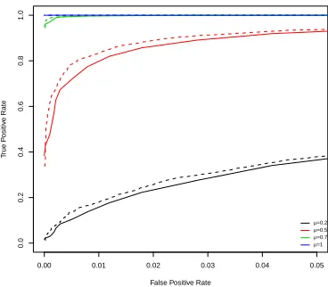
Figure 3.4: Receiver operating curves for (solid line) i.i.d. normal data and (dashed line) correlated normal data (Autoregressive data with parameter 0.8) which exhibits a change in mean from zero to a new mean levelµ.
in a forecasting setting our data will most likely contain autocorrelation structure.
Despite this, the algorithm is still effective at locating changes in mean (Lavielle and
Moulines, 2000).
Figure 3.4 shows the receiver operating curves (ROCs) for detecting a change in mean
both with and without autocorrelation. In this simple example we can see that when
there is autocorrelation present, we have increased power to detect changes. However,
this results in an increased false positive rate. This inflation of the type I error rate
can also be seen in Lund et al. (2007). To remedy this, practically we inflate the
standard penalty chosen as suggested by Lavielle and Moulines (2000).
3.2.2
Forecasting
Once we have detected changes in mean, we can incorporate them into our time series
model using external regressors. Algorithm 1 provides pseudo code for forming a
matrix of regressors based upon the changepoint locations. Having attained a matrix
between these and the data in order to remove the effect of the level shifts. This can
be done independently of the time series model, in which case we would fit the time
series model to the residuals of the linear regression, or it can be done as part of the
modelling process.
Algorithm 1: Incorporating mean changes into forecasts Data: Time series Y = (y1, . . . , yn), xi ∈R
Result: Matrix of external regressors representing mean changes to be used for both model fitting and forecasting.
1 Letτ0 = 0 andτm+1 =m and detect changes in mean τj for j = 1, . . . , m.; 2 if m = 0 then
3 V =N U LL;
4 Vout =N U LL;
5 else
6 V ∈Rm×n;
7 for j ∈[1, . . . , m] do 8 vj,i =
1 i∈(τj−1, τj],
0 otherwise.
9 end
10 Vout = 0m×1;
11 end
12 return V, Vout
In Section 3.4 we test this approach in a simulation study. In the next section, we turn
our attention to an alternative approach to using changepoints to improve forecasts.
3.3
Modelling
For the purpose of forecasting, we wish to detect statistically significant changes in
the model we are using to produce forecasts. Thus, in order to improve forecasts,
we propose to use a cost function, C(·), based upon the log-likelihood of our time series model. In the following, we describe this for the case of using an autoregressive
moving average (ARMA) model for forecasting our time series. For an overview of
(2000).
Suppose the time series we are trying to forecast, {yt}t=1,...,n is not stationary. To
model this non-stationarity, we can segment the data into stationary autoregressive
moving average (ARMA) processes. Let the ith segment of the series, y
τi−1+1:τi, be
modelled by the ARMA(pi,qi) process
yτi−1:τi =µi+
θi(B)
φi(B)
t,i,
whereφi(B) is the autoregressive operator and θi(B) is the moving average operator,
each represented as a polynomial in the backwards shift operator given as
φi(B) = 1−φi,1B−. . .−φi,piB
pi,
θi(B) = 1 +θi,1B+. . .+θi,qiB
qi,
and the noise processt,i is i.i.d. with mean zero and variance σ2i. Note that as well
as allowing both the order of the ARMA model to change, and the coefficients of the
fitted model, we are also allowing for a change in mean level to occur by the inclusion
of µi.
It is often the case that our time series will also have some seasonality structure with
seasonal cycle of lengthf. For example, the GDP data in Figure 3.1 is quarterly data
and we may wish to model this cyclic variation and allow for changes in the
season-ality structure. In this instance, we can model yτi−1+1:τi as a multiplicative seasonal
autoregressive moving average process, denoted ARMA(pi,qi)×(Pi,Qi)f, and write
yτi−1:τi =µi+
θi(B)Θi(Bf)
φi(B)Φi(Bf)
t,i, (3.1)
opera-tors, respectively, given by
Φi(B) = 1−Φi,1Bf −. . .−Φi,piB
f Pi,
Θi(B) = 1 + Θi,1Bf +. . .+ Θi,qiB
f Qi.
In addition to exclusively modelling the response time series, it may also be necessary
to include external regressors into the model. In this situation we model the ith
segment of the series as linear regression model with seasonal ARMA errors. In this
case we have
yt=β0,i+β1,ix1,t+. . .+βk,ixk,t+rt,i, τi−1 < t≤τj,
where the linear regression residuals follow a seasonal ARMA process as in equation
(3.3) andx= (x1, . . . , xk) are the explanatory variables. When the model is estimated,
it is important to remember that we minimize the sum of squared valuest,i, and not
the rt,i.
Having specified the model for each of the segments of our data, we can detect the
locations of changes in the regression model for the time series by incorporating twice
the negative log-likelihood of the model into the optimisation problem in equation
(2.4). Appendix 3.A outlines a procedure for doing this in practice.
3.3.1
Forecasting
Once we have detected changes in the model we are using to forecast, we then forecast
the time series based on the most recent segment of data using the model for that
segment. As a consequence of this approach, once a changepoint has occurred, we are
multiple changepoints we impose a minimum segment length,g, such thatτi+1−τi ≥
g ≥ 2. It important that our minimum segment length is not set so small such we are producing out-of-sample forecasts based only on a small amount of data. In
particular, if the data has seasonality, then we must allow enough observations in a
segment to estimate this seasonality. Also, the longer the minimum segment length,
the more time we have to wait to detect a change. Consequently, we could be fitting
an incorrect model to the last segment of the data therefore introducing bias into
our model. In addition to this, penalty choice is important because it allow us to
control the sensitivity of the changepoint algorithm, if we set it high, then we are
only concerned with macro changes that occur in the data, if we set it low, then we
wish to detect more changes.
The combination of penalty and minimum segment length can have a large influence
on the detected changepoint locations and hence the window we are using to estimate
our forecasting model. The combination of these two allows us to control the trade off
between the bias and variance of our forecasts. As such, in practice, one could
com-pare, or combine, multiple forecasting models based upon the different segmentations
obtained when changing the combination of minimum segment length and penalty.
In the next section, we test the performance of the methodology described here in a
simulation study.
3.4
Simulation Study
In this simulation study we test the performance of using changepoints to improve
forecasts. We compare the following three models:
• M1: A stationary S/ARIMA model;
• M3: A piecewise S/ARMA model.
In order to only access the relative gain from detecting changepoints, a S/AR(I)MA
model is used in all three models. To estimate this model, we use theforecast::auto.arima
function (Hyndman et al., 2007). This could be replaced with an alternative time
se-ries model, for example an exponential smoothing model.
To detect changes in mean for model M2 we use thechangepoint::cpt.meanfunction
(Killick and Eckley, 2014). This function implements the PELT algorithm for a change
in mean under the assumption of Gaussian data. Note that thechangepoint::cpt.mean
function assumes a variance of one. This means that the data should be pre-scaled to
variance one prior to detecting changes in mean.
In order to fit model M3, we adopt the approach outlined in Appendix 3.A.
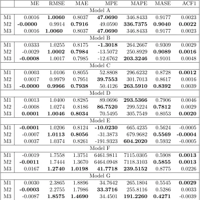
In each instance we simulate 500 realisations of the models and report a selection of
commonly used in-sample and out-of-sample performance metrics:
• Mean Error (ME);
• Root Mean Squared Error (RMSE);
• Mean Absolute Error (MAE);
• Mean Percentage Error (MPE);
• Mean Absolute Scaled Error 1;
• The autocorrelation at lag 1 of the residual errors of the model (ACF1).
Each of these metrics for a model can be attained using the forecast::accuracy
function in R, providing convenient model evaluation for the user. These are reported
in Table 3.1 for the training (in-sample) set and in Table 3.2 for the test
(out-of-sample) set.
1MASE calculation is scaled using MAE of training set naive forecasts for non-seasonal time
ME RMSE MAE MPE MAPE MASE ACF1 Model A
M1 0.0016 1.0060 0.8037 47.0690 346.8433 0.9177 0.0023
M2 -0.0000 0.9914 0.7916 49.0590 336.7375 0.9040 0.0022
M3 0.0016 1.0060 0.8037 47.0690 346.8433 0.9177 0.0023
Model B
M1 0.0333 1.0255 0.8175 -1.3018 264.2667 0.9309 0.0029
M2 -0.0029 1.0002 0.7984 -13.5072 250.8929 0.9089 0.0016
M3 -0.0008 1.0017 0.7985 -12.6762 203.3246 0.9101 0.0048
Model C
M1 0.0003 1.0106 0.8055 52.8808 296.6232 0.8728 0.0012
M2 0.0017 0.9979 0.7951 39.7553 301.7013 0.8617 0.0016
M3 -0.0000 0.9966 0.7938 50.4126 263.5910 0.8392 0.0039
Model D
M1 0.0013 1.0400 0.8285 89.0696 293.5366 0.7906 0.0046
M2 -0.0008 1.0274 0.8186 86.7520 299.5224 0.7812 0.0029
M3 0.0001 1.0046 0.8034 70.5495 305.7549 0.8053 0.0020
Model E
M1 -0.0001 1.0206 0.8124 -10.0230 665.4235 0.5624 -0.0005
M2 -0.0007 1.0113 0.8056 -31.3873 679.9682 0.5569 -0.0004
M3 0.0037 1.0374 0.8261 -191.9323 604.2020 0.5932 -0.0005
Model F
M1 -0.0019 1.7558 1.3751 6461.9811 7115.0305 0.5908 0.0013
M2 -0.0011 1.7444 1.3670 6464.0948 7118.3103 0.5855 0.0013
M3 0.0167 1.2740 1.0198 41.7718 239.5152 0.8775 0.0226
Model G
M1 0.0030 2.3865 1.8896 34.7642 265.1804 0.5545 0.0029
M2 -0.0003 2.2755 1.7986 33.3716 255.8116 0.5286 0.0033
[image:45.612.125.524.155.554.2]M3 -0.0087 1.8575 1.4690 34.4501 191.2260 0.4271 -0.0039
ME RMSE MAE MPE MAPE MASE Model A
M1 -0.1563 1.1671 1.0282 113.3594 169.0906 1.1740
M2 -0.2580 1.3524 1.1853 130.0618 184.9175 1.3521
M3 -0.1563 1.1671 1.0282 113.3594 169.0906 1.1740
Model B
M1 -0.1769 1.1521 1.0119 -17.0005 221.3590 1.1517
M2 -0.2434 1.3917 1.2360 -202.3013 456.4171 1.4062
M3 -0.1411 1.1583 1.0183 -17.8884 206.2740 1.1602
Model C
M1 0.1661 1.0751 0.9265 68.4680 188.4346 1.0055
M2 0.1211 1.1043 0.9442 110.8610 196.6434 1.0249
M3 0.1711 1.0643 0.9143 68.0920 156.3316 0.9695
Model D
M1 0.0313 0.9381 0.7881 102.6425 160.8289 0.7535
M2 0.0325 0.9767 0.8260 129.5255 207.3461 0.7888
M3 0.0354 0.9100 0.7644 76.8555 133.8241 0.7679
Model E
M1 -0.0711 1.1381 0.9713 90.1890 216.4954 0.6714
M2 -0.1162 1.1723 1.0029 100.3486 244.7225 0.6941
M3 -0.0752 1.1093 0.9436 86.3775 201.4708 0.6774
Model F
M1 -0.0669 1.8831 1.6579 117.3606 278.6023 0.7133
M2 -0.1936 2.1786 1.9157 178.7814 263.3264 0.8164
M3 -0.0197 1.7353 1.5182 90.9365 194.1363 1.3165
Model G
M1 -0.1240 2.7002 2.3515 81.9197 142.3822 0.6852
M2 0.0237 6.0104 5.3974 -54.1455 460.6030 1.5817
[image:46.612.154.497.157.551.2]M3 -0.2269 2.1403 1.8835 61.0397 185.1860 0.5466
We simulate 500 realisations from the following scenarios, in which the residual process
is given byt∼ N(0,1).
(a) Stationary AR(2) model with no seasonal components. This scenario is designed to asses the method when there are no changepoints. Specifically, for this
model, we simulate from
Yt= 0.8Yt−1−0.2Yt−2+t, 1≤t≤512.
For scenario (a) the stationary model with mean level changes, M2, produces an
overall better in-sample fit than the other two models. For the test set, the stationary
model (M1) and the piecewise stationary model (M2) produce better out-of-sample
forecasts. Model M2 in this scenario is most likely to over-fit the data, producing a
better in-sample fit but consequently producing worse forecasts. This is because the
presence of autocorrelation can induce features which resemble changes in mean, a
feature previously noted in the literature by Beaulieu et al. (2012). Figure 3.5 shows
a single realisation from scenario (a) along with detected changes in mean. Despite
inflating the penalty to account for the presence of autocorrelation, changepoints are
still detected. Consequently, model M1 over-fits to the level of the time series, and as
a result, will misspecify the autoregressive parameters of the model.
Tables 3.2 and 3.1 for models M1 and M2 are the same to four decimal places, this
suggests a low false positive rate for the change in ARMA model.
0 100 200 300 400 500
−3
−2
−1
0
1
2
3
Figure 3.5: A realisation Yt from scenario (a) with detected changes in mean. We
can see that although there are no ’true’ changes in mean, the autocorrelation causes them to be detected.
simulate from
Yt=
0.8Yt−1−0.2Yt−2+t 1≤t ≤256
2 + 0.8Yt−1−0.2Yt−2+t 256≤t≤512
Overall for scenario (b) model M2 produces a better fit to the training set, this is
expected as it is the most appropriate method to use for the scenario. Out-of-sample
however, model M1 produces the best forecasts. In this case we expect M3 to perform
poorest because it should detect a change in the level of the AR model and then deem
pre-break information uninformative. As a result, the autoregressive coefficients will
be estimated using only a portion of the data.
(c) A piecewise stationary AR(2) model with changing coefficients. Specif-ically, for this model, we simulate from
Yt=
0.8Yt−1−0.2Yt−2+t 1≤t ≤256
0.5Yt−1−0.1Yt−2+t 256≤t≤512
in-sample fit to the data, again we expect this because this model is most in line with
the nature of the behaviour of the time series. In this instance, the results for both
the training and test set support the use of model M3.
(d) A piecewise stationary AR model which changes from a third order to a first order process with a short segment at the beginning of the time series. Specifically, for this model, we simulate from
Yt =
0.1Yt−1−0.6Yt−2−0.3Yt−3+t 1≤t≤50
0.3Yt−1+t 51≤t ≤512
In scenario (d) both the order and the coefficients of the AR model change and model
M3, the piecewise stationary model, can capture this the best producing better
in-sample results, it also achieves better out-of-in-sample forecasts.
(e) A piecewise stationary AR model which changes from a third order to a first order process with a short segment at the end of the time series. Specifically, for this model, we simulate from
Yt=
0.1Yt−1−0.6Yt−2−0.3Yt−3 +t 1≤t ≤462
0.3Yt−1+t 462≤t≤512
In scenario (e) we again have a change in both the order and coefficients of the AR
model, however in contrast to scenario (d), the change occurs at the end of the time
series. Although the piecewise model M3 produces better out-of-sample forecasts than
the stationary model M1, we can see in Table 3.2 that the results differ less than in
scenario (d). This is expected because model (c) has a longer segment which will
produce a better model fit with less variability and thus improved forecasts. For the