Piecewise Deterministic Markov Processes for Continuous Time Monte Carlo

Piecewise Deterministic Markov Processes for Continuous-Time Monte

Carlo

Paul Fearnhead

_{, Joris Bierkens}

_{, Murray Pollock}

_{and Gareth O Roberts}

1

_{Department of Mathematics and Statistics, Lancaster University}

_{DIAM, TU Delft}

3

_{Department of Statistics, University of Warwick}

_{Correspondence: [email protected]}

February 16, 2018

Abstract

Recently there have been conceptually new developments in Monte Carlo methods through the introduction of new MCMC and sequential Monte Carlo (SMC) algorithms which are based on continuous-time, rather than discrete-time, Markov processes. This has led to some fundamentally new Monte Carlo algorithms which can be used to sample from, say, a posterior distribution. Interestingly, continuous-time algorithms seem particularly well suited to Bayesian analysis in big-data settings as they need only access a small sub-set of data points at each iteration, and yet are still guaranteed to target the true posterior distribution. Whilst continuous-time MCMC and SMC methods have been developed independently we show here that they are related by the fact that both involve simulating a piecewise deterministic Markov process. Furthermore we show that the methods developed to date are just specific cases of a potentially much wider class of continuous-time Monte Carlo algorithms. We give an informal introduction to piecewise deterministic Markov processes, covering the aspects relevant to these new Monte Carlo algorithms, with a view to making the development of new continuous-time Monte Carlo more accessible. We focus on how and why sub-sampling ideas can be used with these algorithms, and aim to give insight into how these new algorithms can be implemented, and what are some of the issues that affect their efficiency.

1

Introduction

Monte Carlo methods, such as MCMC and SMC, have been central to the application of Bayesian statistics to real-world problems (Robert and Casella, 2011; McGrayne, 2011). These established Monte Carlo methods are based upon simulating discrete-time Markov processes. For example MCMC algorithms simulate a discrete-time Markov chain constructed to have a target distribution of interest, the posterior distribution in Bayesian inference, as its stationary distribution. Whilst SMC methods involve propagating and re-weighting particles so that a final set of weighted particles approximate a target distribution. The propagation step here also involves simulating from a discrete-time Markov chain.

In the past few years there have been new developments in MCMC and SMC methods based on continuous-time versions of these Monte Carlo methods. For example, continuous-time MCMC algorithms have been proposed (Peters and de With, 2012; Bouchard-Cˆot´e et al., 2017; Bierkens et al., 2017b; Bierkens et al., 2016) that involve simulating a continuous-time Markov process that has been designed to have a target distribution of interest as its stationary distribution. These continuous-time MCMC algorithms were originally motivated as they are examples of non-reversible Markov processes. There is substantial evidence that non-reversible MCMC algorithms will be more efficient than standard MCMC algorithms that are reversible (Neal, 1998; Diaconis et al., 2000; Neal, 2004; Bierkens, 2015), and there is empirical evidence that these continuous-time MCMC algorithms are more efficient than their discrete-time counterparts (see e.g. Bouchard-Cˆot´e et al., 2017). Similarly a continuous-time version of SMC has also been recently proposed (Fearnhead et al., 2016), which involves propagating particles using a continuous-time Markov process. The original motivation for this was to be able to target distributions related to infinite-dimensional stochastic processes, such as diffusions, without resorting to any time-discretisation approximations. However, we show below that one application of this methodology is to generate weighted-samples from a target distribution of interest, giving an alternative interpretation of the recently proposed SCALE algorithm of Pollock et al. (2016a).

The purpose of this paper is to show that continuous-time MCMC and continuous-time SMC methods are linked through the fact that they both are based upon simulating continuous-time processes called piecewise-deterministic Markov processes. These are processes that evolve deterministically between a countable set of random event times. The stochasticity in the process is due to the randomness regarding when these events occur, and possibly random dynamics at the event times. These processes are natural building blocks of continuous-time Monte Carlo methods, as they involve a finite amount of computation to simulate as only a finite number of events and transitions are simulated in any fixed time-interval.

make the development of new continuous-time Monte Carlo methods more accessible and help stimulate work in this area.

One aspect of continuous-time Monte Carlo that is particularly relevant for modern applications of Bayesian statistics is that they seem well-suited to big-data problems. If we denote our target distribution byπ(x) then the dynamics of these methods depend on the target through∇logπ(x). Now ifπ(x) is a posterior distribution, then it will often be in product-form, where each factor relates to a data-point or set of data-points. This means that ∇logπ(x) is a sum, and hence is easy to approximate unbiasedly using sub-samples of the data. It turns out we can use these unbiased estimators within the continuous-time Monte Carlo methods without affecting their validity. That is, the algorithms will still target π(x). This is in comparison to other discrete-time MCMC methods that use sub-sampling (Welling and Teh, 2011; Bardenet et al., 2017; Ma et al., 2015; Quiroz et al., 2015), where the approximation in the sub-sampling means that the algorithms will only target an approximation to π(x). It also compares favourably with big-data methods that independently run MCMC on batches of data, and then combines the MCMC samples in some way (Neiswanger et al., 2014; Scott et al., 2016; Srivastava et al., 2015; Li et al., 2017). As the combination steps involved will also introduce some approximation error.

The outline of the paper is as follows. In the next section we give an informal introduction to Piecewise Deter-ministic Markov processes. Our aim is to cover key relevant concepts linked to these processes whilst avoiding technical details. Those interested in a more rigorous introduction should see Davis (1984) and Davis (1993). Sections 3 and 4 then cover continuous-time versions of MCMC and SMC respectively. These have been written so that either section could be read independently of the other. Our aim for each section is to introduce the continuous-time Monte Carlo algorithm, show how it relates to a piecewise deterministic Markov process, and how we can use the theory for these processes to see that the Monte Carlo algorithms target the correct dis-tribution. We also cover how these algorithms can be implemented using sub-sampling ideas, and highlight the importance of low-variance sub-sampling estimators for obtaining highly efficient samplers for big-data.

2

Piecewise Deterministic Markov Processes

The continuous-time versions of SMC, or sequential importance sampling, and MCMC that we will consider later are all examples of time-homogeneous piecewise-deterministic Markov processes. We will henceforth call these piecewise deterministic processes or PDPs.

A PDP is a continuous-time stochastic process. Throughout we will denote the state of a PDP at time t by

Zt. The dynamics of the PDP involves random events, with deterministic dynamics between events and possibly

random transitions at events. These dynamics are thus defined through specifying three quantities:

equation:

dz_t(i)

dt = Φi(zt), (1)

fori= 1, . . . , d, for some known vector-valued function Φ = (Φ1(z), . . . ,Φd(z)). This will lead to a

deter-ministic transition function, so that the solution of the differential equation starting from valueztand run

for a time interval of lengthswill give

zs+t= Ψ(zt, s)

for some function Ψ.

(ii) The event rate. Events will occur singularly at a rate,λ(zt), that depends only on the current position

of the process. The probability of an event in interval in [t, t+h] given the state at time t, zt, is thus

λ(zt)h+o(h).

(iii) The transition distribution at events. At each event the state of the process will change, according to some transition kernel. For an event at timeτ, ifzτ− denotes the state immediately prior to the event,

then the state at timeτ will be drawn from a distribution with densityq(·|zτ−).

To define a PDP process we will also need to specify its initial condition. We will assume thatZ0 is drawn from some known distribution with density function p0(·).

2.1

Simulating a PDP

To be able to use a PDP as the basis of an importance sampling or MCMC algorithm, we will need to be able to simulate from it. A general approach to simulating a PDP is to iterate the following steps:

(S1) Given the current time,t, and state of the PDP,zt, simulate the next event time,τ say.

(S2) Calculate the value of the process immediately before the next event time

zτ−= Ψ(zt, τ−t).

(S3) Simulate the new value of the process, immediately after the event, fromq(zτ|zτ−).

The simulation algorithm is initiated with a current time t= 0 and withZ0 drawn from the initial distribution of the process. To simulate the process for a time intervalT these steps can be iterated until the first event time after T. If we wish to then simulate the value of the process at a time, s say, between events we just find the event time,τ, immediately prior tos; the value of the process immediately after the event,zτ; and then set

Ifsis a time before the first event we would useτ= 0.

Below we will assume that our PDP has been chosen so that Ψ(·,·) is known analytically and that the proposal distribution at events, q(·|·), can be easily simulated from. Thus the only challenging step to simulating a PDP will be simulating the next event in step S1. This involves simulating the next event in a time-inhomogeneous Poisson process.

The first thing to note is that the event rate in (S1) can be written as a deterministic function of time, as the state dynamics are deterministic until the next event. If we are currently at time t with state zt, then for any

future timet+sbefore the next event, the state will bezt+s= Ψ(zt, s). Thus the event rate will be

λ(zt+s) =λ(Ψ(zt, s)) = ˜λzt(s),

for a suitably defined function ˜λzt(·). We can simulate the time until the next event, s, as the time of the first

event in a Poisson process of rate ˜λzt(u).

If the event rate is a simple function, then we can simulate events directly. Define Λz(s) =

∫s

0 λ˜z(u)du. We simulate a the time of an event,ssay, by (i) simulatingu, the realisation of an exponential random variable with rate 1, and (ii) findings >0 the solution of Λz(s) =u(e.g. Cinlar, 2013).

For more complicated rate functions either calculating Λz(s) or solving the equation in step (ii) may not be

tractable. In such cases the most general approach to simulating event times is by thinning, or adaptive thinning (e.g. Lewis and Shedler, 1979).

If we can upper-bound the event rate, ˜λzt(u) < λ

+_{(u), then thinning works by simulating possible events of}

a Poisson process of rate λ+(u) and accepting a possible event at time u as an actual event with probability ˜

λzt(u)/λ

+_{(u). The time of the first accepted event will be the time until the next event for our PDP. This requires}

the upper boundλ+_{(u) to be such that simulating events from a Poission process of rateλ}+_{(u) is straightforward} – for exampleλ+_{(u) is constant or linear inu, or piecewise constant or piecewise linear. Obviously the lower the} boundλ+ _{the more computationally efficient this approach will be.}

2.2

Analysing a PDP

continuous-time Monte Carlo methods. For further details on generators see Section 14 of Davis (1993), and for further information on calculating the invariant distribution if a PDP see Section 34 of Davis (1993).

2.2.1 The Generator

The generator of a continuous-time, time-homogeneous, Markov process is an operator that acts on functions of the state variable. We will denote the generator by A. For suitable functionsf(z), the generator is defined by

Af(z) = lim

δt_→0

E(f(Zt+δt)|Zt=z)−f(z)

δt .

The set of suitable functions, which are the functions for which this limit exists for allz, is called the domain of the generator.

The fact that the process is time-homogeneous means that the right-hand side does not depend on t. We can interpret the generator applied to a functionf(z), as giving the derivative of the expectation off(Zt) conditional

on the current value of Zt. As the generator specifies how the expectation of any suitable functionf(·) changes

over time, it uniquely defines the dynamics of the underlying continuous-time stochastic process, in a similar way that knowing the moment generating function of a random variable will uniquely determine its distribution (Ethier and Kurtz, 2005).

If we are interested in the derivative of the expectation of a function of our PDP at a time t, then we can write this as

dE(f(Zt))

dt = limδt→0

E(f(Zt+δt)−E(f(Zt))

δt = limδt→0Et

(

Et+δt|t(f(Zt+δt)|Zt)−f(Zt)

δt

)

,

where in the last expression the inner expectation is with respect to Zt+δt given Zt and the outer expectation

with respect toZt. Assuming we can exchange the outer expectation and the limit we get

dE(Zt)

dt = Et(Af(Zt)). (2)

Thus the derivative of the expectation of our function is the expectation of the generator applied to the function.

Davis (1984) gives the generator for a piecewise deterministic process:

Af(z) = Φ(z)· ∇f(z) +λ(z)

∫

q(z′|z)[f(z′)−f(z)]dz′, (3)

for functions f(·) such that t 7→ f(Ψ(z, t)) is absolutely continuous. The form of the generator has a simple interpretation. The first term on the right-hand side relates to the deterministic dynamics. For deterministic dynamics the generator is just the time-derivative of f(zt), which by the product rule is

df(zt)

dzt

=

d

∑

i=1

∂f(zt)

∂z(ti)

∂z(ti)

where Φ(z) is defined in (1). The second term on the right-hand side is the change in expectation at events. The probability of an event in time [t, t+h] isλ(zt)h+o(h) and the change in expectation conditional on event

occuring, up to terms ofo(h), is given by the integral on the right-hand side.

2.2.2 The Forward Operator and Fokker-Planck Equation

We can define the adjoint of a generator of a continuous-time Markov process,A∗, such that for suitable functions

g(z) andf(z)

∫

g(z)Af(z)dz=

∫

f(z)A∗g(z)dz.

Now if we define the density function of our continuous-time Markov process at timet to bept(z) then from (2)

we get that, for suitable functionf, the derivate of the expectation off(Zt) with respect tot is

dE(Zt)

dt = Et(Af(Zt)) =

∫

pt(z)Af(z)dz=

∫

f(z)A∗pt(z)dz.

However we can equally write this derivative as

dE(Zt)

dt =

d dt

∫

pt(z)f(z)dz=

∫

∂pt(z)

∂t f(z)dz,

again assuming we can interchange differentiation and integration. This gives that

∫

dpt(z)

dt f(z)dz=

∫

f(z)A∗pt(z)dz.

As this holds for sufficiently many functionsf(z) we get

∂pt(z)

∂t =A

∗_p

t(z).

This is a partial differential equation for the distribution of the stochastic process, known as the Fokker-Planck or Forward Kolmogorov equation.

It is straightforward to show that the adjoint of the generator of a PDP (3) is

A∗_{g(z) =−}

d

∑

i=1

∂Φi(z)g(z)

∂z(i) +

∫

g(z′)λ(z′)q(z|z′)dz′−g(z)λ(z) (4)

Ifp(z) is an invariant distribution of our PDP than it will satisfyA∗p(z) = 0, which gives

−

d

∑

i=1

∂Φi(z)p(z)

∂z(i) +

∫

p(z′)λ(z′)q(z|z′)dz′−p(z)λ(z) = 0.

The first term here relates to the change in probability mass caused by the deterministic dynamics, the second term relates to the probability flow into state zand the final term the probability flow out of state z. For an invariant distribution these will cancel for all statesz.

3

Continuous-Time MCMC

We first consider continuous-time versions of MCMC. These algorithms involve simulating a PDP process which has a given target distribution, π(x), as its stationary distribution. Such algorithms were originally of interest as they are reversible processes. As mentioned in the introduction, there is substantial evidence that non-reversible MCMC algorithms are more efficient than standard, non-reversible MCMC. Intuitively this is because non-reversible MCMC suppresses the random-walk behavour of reversible MCMC and thus can more rapidly explore the state-space. Furthermore it has been shown that continuous-time MCMC is suitable for using sub-sampling ideas, similar to those in Section 4.3. Thus these methods are also promising for big-data applications of MCMC.

3.1

The Continuous-time limit of MCMC

To help build intuition for continuous-time MCMC, and to see how it links to discrete-time MCMC algorithms, we will first derive a continuous-time algorithm as a limiting form for a simple non-reversible discrete-time MCMC algorithm (Gustafson, 1998; Diaconis et al., 2000). This MCMC algorithm will target a joint distribution of (x,v), where v can be viewed as a velocity. For our specific algorithm we will consider only velocities of a fixed, say unit, speed, and hencevcould equally be defined as a direction. Our MCMC will target a distributionπ(x)pu(v)

wherepu(v) will be the uniform distribution over all velocities with unit speed.

The MCMC algorithm will have two types of move. The first involves two deterministic proposals

(1a) Propose a move from (x,v) to (x+hv,−v). Accept this with the standard Metropolis-Hastings accept probability, which simplifies to

min

{

1,π(x+hv) π(x)

}

(1b) Move from (x′,v′) to (x′,−v′).

again. So the net affect of applying both (1a) and (1b) is that the velocity is unchanged if we accept the proposed move in step (1a) but flips if we reject the move. This is a standard approach in Hamiltonian Monte Carlo (Neal et al., 2011). In fact this algorithm can be viewed as a type of Hamiltonian Monte Carlo move, but based on the dynamics of an approximate potential forxwhich is uniform (and hence the velocity is not changed other than by the flip).

Whilst this move keepsπ(x)pu(v) invariant, it leads to a reducible Markov chain if the dimension ofxis greater

than 1, as it only proposes moves along the direction given byv. Thus we need a second type of move to produce an irreducible MCMC algorithm with the required asymptotic distribution. The second move we use is an update of v, from some transition kernel that has pu(v) as its stationary distribution. We will imagine applying N

transitions of type 1 between each of these updates just ofv.

Under this framework we can then consider letting h→0 while keepings=hN a constant. We will scale time so that theith MCMC transition will occur at timeih, and define (xt,vt) to be the value of the state after the

ith MCMC transition for ih≤t <(i+ 1)h.

Now for each move in step (1a) the rejection probability for smallhis

max{0,1−exp[logπ(x+hv)−logπ(x)]}= max{0,1−exp[v· ∇logπ(x)h+o(h)]}= max{0,−v· ∇logπ(x)h}+o(h),

assuming that, for example,π(x) is twice differentiable.

Thus in our limit as h→0, rejections in step (1a) will occur as events in a Poisson process of rateλ(xt,vt) =

max{0,−vt· ∇π(xt)}. The dynamics between these events will be deterministic, withvt being constant andxt

changing as in a constant velocity model with velocity vt. At each event the velocity will just flip. Note that

while the process is moving to areas of higher probability density, as defined by π(x), the rate of the Poisson process will be 0. Thus events will only occur if the process is moving to areas of lower probability mass.

This limiting process is just a PDP with constant velocity dynamics between events, with the velocity changing at event times.

It is natural to consider a general class of PDP processes with these dynamics, and see what flexibility there is in choosing the distribution of the event times, and the distribution of the change of velocity at events, so that we still have a process whose marginal stationary distribution forXt isπ(x). To do this, denote the state of our

PDP byZt= (Xt,Vt), and assume our PDP has the following dynamics:

(i) The deterministic dynamics. Fori= 1, . . . , d

dx(_ti)

dt =v

(i)

t , and

dv_t(i)

dt = 0.

(ii) The event rate. Events will occur at a rate,λ(zt).

(iii) The transition distribution at events. At an event at timeτ, xτ =xτ− and vτ is drawn from some

transition densityq(·|xτ−,vτ−).

We now need to consider how to choose the event rate and the transition density so that π(x) is the marginal stationary distribution.

3.2

The Stationary Distribution of the PDP

A necessary condition forπ(x) to be the marginal stationary distribution of our PDP is that it is the marginal of an invariant distribution for the PDP. We will use the adjoint of the generator of our PDP to derive a condition on both the event rate and the transition distribution at events for the PDP to haveπ(x) as the marginal of an invariant distribution.

As above, let z = (x,v). Denote the invariant distribution of our PDP by p(z). We can factorise this as the product of the marginal stationary distribution for x times the conditional forv given x, and we wish to have

p(z) =π(x)p(v|x). If A∗ is the adjoint of the generator of our PDP, asp(z) in an invariant distibution we have

A∗_{p(z) = 0. This gives}

−π(x)p(v|x)[v· ∇xlogπ(x) +v· ∇xlogp(v|x) +λ(z)] + ∫

λ(x,v′)q(v|x,v′)π(x)p(v′|x)dv′= 0. (5)

In the above∇xdenotes the vector of first partial derivative with respect to the components ofx.

To date, all continuous-time MCMC algorithms have been designed so that under the invariant distributionv is independent ofx, and thus all components of∇xlogπ(v|x) will be 0. If we wish to design such a process we need

to chooseλ(x,v) andq(v′|x,v) such that, by rearranging (5),

pv(v)λ(x,v)−

∫

λ(x,v′)q(v|x,v′)pv(v′)dv′=−pv(v)v· ∇xlogπ(x), (6)

for some distributionpv(v) for the velocity. The left-hand side is measuring the net probability flow out of states

with velocity v, this must offset the change in probability mass for V caused by the deterministic dynamics, which is the term on the right-hand side.

Note that if we integrate (6) with respect to v, the left-hand side is 0. So we get E(V)· ∇logπ(x) = 0, where the expectation is with respect to the invariant distribution for the velocity. As this will need to hold for allx, we can see that the invariant distribution for all components of the velocity must have zero mean.

The actual processes we describe in the next section all allow velocities within some symmetrical set, and are designed so that pv(v) is uniform on this set. They ensure (6) holds through deterministic dynamics at events.

only allow transitions between pairs of velocities, v and v′ that satisfy v′ = Fx(v) and, by definition of Fx,

v=Fx(v′). Under this constraint on the transitions at events we get a simple set of equations that we need the

event rates to satisfy. For anyv, and withv′=Fx(v), it is straightforward to show that (6) holds if and only if

λ(x,v)−λ(x,v′) =−v· ∇xlogπ(x). (7)

for allx. Note that as this equation must also hold forv′, we immediately see that only flip operators for which

Fx(v)· ∇xlogπ(x) = −v· ∇xlogπ(x) are allowable. The rates only depend on the target through the term

∇xlogπ(x), which means thatπ(x) is only needed to be known up to proportionality. Also note that (7) does

not uniquely define the rates. If we have a set of rates,λ(x,v) that satisfy (7), then λ(x,v) +γ(x,v) will also satisfy (7) for any positive functionγ(x,v) for which γ(x,v) =γ(x, Fx(v)).

A natural choice of rates which satisfy (7) are those which are smallest. This will give λ(x,v) = max{0,−v·

∇xlogπ(x)}. We will call these thecanonical rates. Theoretical justification for the canonical rates whend= 1

is given in Bierkens and Duncan (2017), who show that the asymptotic variance of Monte Carlo estimators is minimised when using these rates.

3.2.1 Different continuous-time MCMC algorithms

We now describe a number of choices of flip operator, and the corresponding PDPs. We start with the limiting process we derived in Section 3.1, and then describe two continuous MCMC processes that have been recently proposed. These three choices all lead to identical PDPs for a one-dimensional target, but differ in terms of how they extend to higher dimensions. Each assume the target is defined on an unbounded domain; for extensions of these methods to bounded domains see Bierkens et al. (2017a). We will finish with some discussion of alternative schemes that are possible.

Pure Reflection and Refresh

The continuous-time limit we derived in Section 3.1 corresponds to Fx(v) =−v, with the canonical rates. Such

a process we call a pure reflection process. For a multi-dimensional target distribution, this process would be reducible, as it can only explore positionsxthat lie on a straight-line defined by the initial velocity. As such this is an example whereπ(x) would be a marginal invariant distribution but not the marginal stationary distribution. To overcome this we would need an additional move, which refreshes v. Such a refresh move would need to have

pu(v) as its stationary distribution. The times of refreshing could be either deterministic or random.

Bouncy Particle Sampler

It does this by defining Fx(v) to be

Fx(v) =v−2

v· ∇logπ(x)

∇logπ(x)· ∇logπ(x)∇logπ(x). (8)

This flips the component of v that is in the direction of ∇logπ(x) but leaves the components of v that are orthogonal to∇logπ(x) unchanged. They again use the canonical rates. As with the pure reflection process this means that events only occur if the PDP is moving to areas of lower probability mass according to π(x).

The original sampler of Peters and de With (2012) just simulates this PDP. However Bouchard-Cˆot´e et al. (2017) shows that, for some targets, such a sampler can be reducible. This means that, depending on how the process is initiated, there may be parts of the state-space that the Bouncy Particle Sampler cannot reach. As a result the invariant distribution, π(x), of the PDP may not be its unique asymptotic distribution.

The Bouncy Particle Sampler introduces refresh events. Refresh events occur as events of an independent Poisson process of constant rate, and at a refresh event we simulate a new velocity from pv(v). Bouchard-Cˆot´e et al.

(2017) show that for any non-zero rate of this refresh process, the resulting sampling will haveπ(x) as its unique asymptotic distribution.

Zig-Zag Sampler

The Zig-Zag sampler (Bierkens et al., 2017b; Bierkens et al., 2016) considers a discrete set of velocities. If x is

d-dimensional, thenv=∑d_i=1θiei, where eachθi ∈ {−1,1} and e1, . . . ,ed are a set of orthogonal basis vectors

forRd_{. The invariant distribution forvis defined as the uniform distribution over this set of 2}d _{possible values.}

The Zig-Zag sampler can be viewed as having d-distinct event types, each with its own rate, and each with its own deterministic change to the velocity. The ith event will have a flip,F(i), that switchesθi to−θi, but keeps

the velocity in the otherd−1 directions unchanged. If we denoteλi(x,v) to be the rate of events of type i, then

this corresponds to our general formulation of a PDP but withλ(x,v) =∑d_i=1λi(x,v), and with the transition

distribution at an event being a discrete distribution over thedtransitions that correspond to theddifferent flips. Flip i occurs with probabilityλi(x,v)/λ(x,v). Subsituting this into (6) shows that we need to chooseλi(x,v)

so that

d

∑

i=1

{

λi(x,v)−λi(x, F(i)(v))

}

=−

d

∑

i=1

θi

∂logπ(x)

∂x(i) .

Here we have assumed thatx(i)_{is the component ofxin directione}

i. This can be achieved if we choose the rates

such that

λi(x,v)−λi(x, F(i)(v)) =−θi

∂logπ(x)

∂x(i) .

As above, this does not uniquely define the rates, only the difference between rates for velocities that differ in terms of their component in theei direction.

that the Zig-Zag process is ergodic in any of the following cases: (i) one-dimensional target distributions, (ii) factorized target distributions, and (iii) switching rates that are positive everywhere (which can be obtained by adding a constant ε > 0 to the canonical switching rates). Experiments suggest that ergodicity holds in much more generality.

Note that the above argument easily generalises to allowing velocities of the form v=∑m_i=1θiei, where theei

are not constrained to be orthogonal, and we can even allow m > ddirections. Whether there are advantages in using such a set of possible velocities is not clear.

Alternatives

There is substantial extra flexibility in choosing the event rates and the type of transition at events beyond the three examples we have detailed. For example we could consider transitions at an event that does not depend on the current velocity. If we allow v to be any unit vector, then it is straightforward to show that choosing

λ(x,v) = max{0,−v· ∇xlogπ(x)}, and, at each event, sampling a new velocity from the distribution

q(v′|x,v)∝max{0,v′· ∇xlogπ(x)},

will lead to a PDP with invariant distribution that hasπ(x) as its marginal.

More substantial alternatives are also possible. For example, we could consider processes which allow the invariant distribution of Vto depend on x– something that Girolami and Calderhead (2011) has shown to be beneficial for Hamiltonian Monte Carlo methods. For a proposed distribution π(v|x) we would then need to find a set of event rates and transitions that satisfy (5).

3.3

Simulation and Use of Skeletons for Continuous MCMC

So far we have described a number of different PDPs that will haveπ(x) as their marginal invariant distribution. For these to be useful in practice, we need to be able to simulate them efficiently. How to do this in practice will depend on the form ofπ(x), but is likely to use the ideas briefly described at the end of Section 2.1. For further detail see the discussion of this, and suggestions, in Bouchard-Cˆot´e et al. (2017) and Bierkens et al. (2016).

The output of simulating a PDP will be a set of event times and the values of the state at those event times. We wish to use this output to obtain Monte Carlo estimates of expectations of functions ofX, whereXis distributed according to π(x). Assume we have simulated the PDP for some time-interval T. We will discard the value of the process in some burn-in period of lengthtb. Assume there wereN events in the time-interval [tb, T]. Denote

these asτi fori= 1, . . . , N, and letτ0=tb andτN+1=T.

The first is to calculate the average of this function along the path of the PDP:

1

τN+1−τ0

N

∑

i=0

∫ τi+1−τi

0

g(xτi+svτi)ds.

Here each integral corresponds to the integrals of g(xt) for t in [τi, τi+1], and uses the fact that for such a t,

xt=xτi+ (t−τi)vτi.

The above approach is difficult if the integrals are not easy to evaluate. In this case we can resort to a standard Monte Carlo approximation. Choose an integerM >0, defineh= (τN+1−τ0)/M and then use the Monte Carlo estimator

1

M

M

∑

j=1

g(xτ0+jh),

where we can trivially calculate xτ0+jh using the set of event times and the values of the PDP at those event

times.

3.4

Example: Robust Regression

To demonstrate the difference between the Bouncy Particle Sampler and the Zig-Zag sampler, and to compare these methods with more traditional MCMC methods, we will consider their application to a robust regression model. We model the mean of each data point as a linear function ofd−1 covariates and an intercept, but model the errors as a mixture of a standard normal random variable and a normal random variable with mean equal to 0 but a variance equal to 102. Appendix A gives details of the log-posterior for this model and how we can bound the event rate of, and hence simulate events for, either the Bouncy Particle or Zig-Zag sampler.

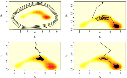
We first compare the dynamics of the Zig-Zag algorithm and the Bouncy Particle Sampler. To do this we consider thed= 2 case, so that we have a bivariate target distribution whose contours we can plot. We simulated

n = 500 data points, with the covariates values being independent draws from a standard normal distribution. We simulated half the data points with parameter values (2,1) and half with parameter values (6,1), with the simulated residuals being from a standard normal distribution. This choice was made so as to produce a posterior distribution with multiple modes – corresponding to the intercept term being either 2, 6, or 4, the average of these values.

1 2 3 4 5 6 7

−1

0

1

2

3

4

β1 β2

2 3 4 5 6

0.5

1.5

2.5

3.5

β1 β2

2 3 4 5 6

0.5

1.5

2.5

3.5

β1 β2

2 3 4 5 6

0.5

1.5

2.5

3.5

β1 β2

Figure 1: Plots of output from the Bouncy Particle Sampler (top-row and bottom-left) and Zig Zag algorithm (bottom-right) for the robust regression model with d= 2. In each case we plot the continuous-time output of the position component of each sampler on top of a heat-map of the posterior for the two parameters (which are denotedβ1, β2). The Bouncy Particle sample output is for different refresh rates: no refresh event (top-left) refresh rate 1 (top right) and refresh rate 100 (bottom left).

where setting the refresh rate to 0 leads to a sampler which is reducible, and, depending on the initial conditions, will not be able to reach some parts of the state-space. By comparison if we use a refresh-rate that is too high (bottom-left) then the resulting process resembles a reversible MCMC algorithm and thus loses the potential advantages of non-reversible dynamics that we obtain with a more reasonable choice of refresh rate (top-right plot). Notice that the Zig-Zag sampler’s dynamics (bottom-right) are qualitatively similar to the Bouncy Particle Sampler’s dynamics when a reasonable refresh rate is chosen. Though the Zig-Zag sampler is restricted to move in certain directions, with the resulting “zig-zag” nature of the output giving the algorithm its name.

We now compare the Bouncy Particle Sampler to a Metropolis adjusted Langevin Algorithm (MALA, Roberts and Rosenthal, 1998), and consider how the two methods compare in both a low-dimensional, d= 8, and high-dimensional,d= 128, setting. We simulated the covariates for each observation from an AR(1) process with lag-1 correlation of 0.5. In both cases we set all co-efficients in the linear model to 0 except for those associated with the intercept and first covariate. We simulated 500 observations, 300 from a model with (β1, β2) = (2,1) and 200 from a model with (β1, β2) = (6,1), and with standard normal residuals in each case. This produces a complex log-posterior whilst ensuring that the log-posterior has a single main mode, which means that auto-correlation summaries of MCMC output are more reliable for estimating the efficiency of the algorithm. We tuned the MALA algorithm to have an acceptance probability close to 0.5 (Roberts and Rosenthal, 1998), and run both MALA and the Bouncy Particle Sampler so that they each had 50,000 iterations (where an iteration for the Bouncy Particle Sampler corresponds to a proposed event-time). The resulting samplers had similar computational costs, with MALA taking slightly longer. For each sampler we removed the first 40% of the output as burn-in. For the Bouncy Particle Sampler we then sampled 30,000 values of the parameters at equally spaced time-points, so that both algorithms gave an identical form of output.

0 10 20 30 40 50

0.0

0.4

0.8

Lag

A

CF

MALA d=8

0 10 20 30 40 50

−0.5

0.0

0.5

1.0

Lag

A

CF

BPS d=8

0 100 200 300 400 500

0.0

0.4

0.8

Lag

A

CF

MALA d=128

0 100 200 300 400 500

0.0

0.4

0.8

Lag

A

CF

BPS d=128

Figure 2: Auto-correlation plot for the intercept parameter from a run of MALA (top-row) and the Bouncy Particle Sampler (bottom-row), ford= 8 (left-column) andd= 128 (right-column).

the low-dimesional case (see left-hand column). However the Bouncy Particle Sampler shows negative auto-correlation. We believe this is caused by the sampler’s dynamics which tends to move from one tail of the posterior to the other (behaviour that is particularly pronounced for 1-dimensional unimodal target distributions; see Bierkens and Duncan, 2017). As a result of this negative correlation, estimates of the auto-correlation time for the Bouncy Particle Sampler are slightly small than for MALA. However, as the dimension increases, we tend to see bigger advantages from using the Bouncy Particle Sampler – perhaps due to its non-reversible dynamics. This can be seen from the auto-correlation plots for d = 128 (see right-hand column). For this run of the two algorithms the estimated auto-correlation times are approximately 670 for MALA and 130 for the Bouncy Particle Sampler, suggesting a 5-fold gain in efficiency from using the latter algorithm. Key to the strong performance of the Bouncy Particle Sampler for this example is the fact that we can efficienctly simulate the event times using thinning – with the method described in Appendix A; with around 30% of proposed event times being accepted.

3.5

Exact Approximation versions and Subsampling

Exact approximate algorithms (Andrieu and Roberts, 2009) are MCMC algorithms that use estimators of the target distribution within the accept-reject step. If implemented correctly, and if these estimators are both positive and unbiased, then it can be shown that the resulting MCMC algorithms are exact: in the sense they still have the target distribution as their stationary distribution. It turns out that exact approximate versions of the continuous-time MCMC algorithms detailed in the previous section are also possible.

3.5.1 Exact Approximation for Pure Reflection and Zig Zag

For the Pure Reflection process the requirement on the rates of events is that for any velocityv

λ(x,v)−λ(x,−v) =−v· ∇logπ(x).

For a given choice of rates, such as the canonical rates λ(x,v) = max{0,−v· ∇logπ(x)}, we would often use thinning to simulate the event times (see Section 2.1). Thus if our current state is (xt,vt) we would introduce a

bound on the event rate fors >0

˜

λ+(s)≥λ(xt+svt,vt),

simulate potential events at rate ˜λ+(s) and accept them with probabilityλ(x+sv,v)/˜λ+(s). The time until the next event is just the time until the first accepted event.

Now assume we have a estimator of−∇logπ(x), which we will denoteU(x). This estimator is a random variable, and examples of how it could be constructed are given below. We further introduce a random rate function

ˆ

λ(x,v) = max{0,v·U(x)}.

This is just the canonical event rate, but replacing −∇logπ(x) with its unbiased estimator. The idea of an exact-approximate version is to simulate events using thinning, with a bound on the event rate that satisfies

˜

λ+(s)≥λˆ(xt+svt,vt)

almost surely, and where we accept points using the random acceptance probability ˆλ(xt+svt,vt)/λ˜+(s).

As the overall acceptance probability will be the expectation of the random acceptance probability, it is straight-forward to show that simulating events in this way is equivalent to simulating events at a rate

λ(x,v) = E (max{0,v·U(x)}), (9)

where expectation is with respect to the random variable U(x). Furthermore if we now calculate the difference in rates, λ(x,v)−λ(x,−v), we have

λ(x,v)−λ(x,−v) = E (max{0,v·U(x)})−E (max{0,−v·U(x)})

= E (max{0,v·U(x)} −max{0,−v·U(x)})

= E (max{0,v·U(x)}+ min{0,v·U(x)}) = E (v·U(x)).

Thus providedU(x) is an unbiased estimator of−∇logπ(x), the resulting process will haveπ(x) as its marginal invariant distribution.

general, be less efficient. This loss of efficiency comes first as the rates that are used for events, E(max{0,v·U(x)}), will, in general, be larger than the canonical rates. The only exception being if U(x) has the same sign as

−∇logπ(x) with probability one. Using larger rates appears to reduce the rate of mixing of the process (see

Bierkens and Duncan, 2017; Bierkens et al., 2016). A related issue is that the bound on the rates, used when implementing thinning, will also tend to be larger. This will increase the cost of simulating the process. Intuitively we would expect both these losses of efficiency to increase as the variability of our estimator increases.

3.5.2 Exact Approximation for the Bouncy Particle Sampler

The idea of an exact approximation version of the Bouncy Particle Sampler is slightly more complicated, due to the fact that the flip operator used also depends on ∇logπ(x). To implement such an exact approximation version we need to use the same estimate of ∇logπ(x) in the flip operator as was used in deciding to accept the event. So, using the notation of the previous section, at a potential event at time s, simulated from a Poisson process with rate ˜λ+_{(s) we will now:}

(1) Simulate u, a realisation ofU(xt+svt).

(2) Accept the event with probability

ˆ

λ(xt+svt,vt)

˜

λ+_(s) =

max{0,u·vt}

˜

λ+_(s)

(3) If we accept the potential event, this corresponds to an event at timet+s, with new state being xt+s=

xt+svt and

vt+s=vt−2

vt·u

u·uu.

Note that the same realisation,u, is used in both steps (2) and (3).

This leads to an algorithm where the transition at an event is random. We will assume that U is a discrete random variable, which is consistent with the use of sub-sampling discussed in Section 3.5.3. It is straightforward to show that the resulting PDP has events occurring at rate (9) as before, but with a transition probability mass function at an event that is

q(v′|x,v) =p(u|x) max{0,u·v} E (max{0,v·U(x)})

3.5.3 Use of Subsampling

An example of an exact-approximate version of these continuous-time MCMC algorithms arises if we use sub-sampling of data points at each iteration when performing Bayesian inference in a big-data setting. This was first suggested for the Zig Zag algorithm by Bierkens et al. (2016). Bouchard-Cˆot´e et al. (2017) has shown that sub-sampling can be used within the Bouncy Particle Sampler (see also Pakman et al., 2017), though they derive this as a special case of what they call the local Bouncy Particle Sampler. This local Bouncy Particle Sampler also allows efficient implementation when the target can be written as a product of factors, each of which only depends on a few components of x.

We will consider a target density of the form

π(x)∝

n

∏

i=1

πi(x).

In this case, the simplest unbiased estimator of−∇logπ(x) is just

−n∇logπI(x), (10)

whereI is drawn uniformly from 1, . . . , n. However, to increase the efficiency of sub-sampling methods we would want to try and minimise the variance of our estimator, for example by using control variates. One approach that is commoly used (e.g. Bardenet et al., 2017; Dubey et al., 2016; Baker et al., 2017) is to have a pre-processing step that finds ˆx, a value ofxthat is near the posterior mode. We then calculate and store ∇logπ(ˆx), and use the following estimator

−∇logπ(ˆx) +n(∇logπI(ˆx)− ∇logπI(x)). (11)

Ifxis within a distance ofO(1/√n) of ˆxand ifπ(x) is sufficiently smooth we would expect the variance of this estimator to only increase linearly with n. By comparison the variance of the simple estimator (10) will increase like O(n2).

3.6

Example: Mixture Model

To demonstrate some of the properties of the use of sub-sampling within continuous-time MCMC algorithms we apply them to a simple mixture model. Assume we have IID data from a mixture distribution, where for

j= 1. . . , n

Yj∼

    

N(0,102_{) with probability p,} N(x,12_{) otherwise.}

This involves inference for a univariate parameter, and for this case each of the three versions of continuous-time MCMC introduced earlier are equivalent. Furthermore we do not need to introduce any refreshing of the velocity, as used within the Bouncy Particle Sampler, to ensure ergodicity (Bierkens and Duncan, 2017). Our aim is to show how the continuous-time MCMC algorithms can be implemented, how the choice of the bounding process that simulates potential event times can affect efficiency, and give some insight into how and when the subsampling ideas can lead to gains in efficiency.

We will first look at implementing continuous-time MCMC using a global bound on the event rates. For this model, if we writeπ(x)∝∏n_i=1πi(x), where πi is the likelihood of the ith observation times the 1/nth root of

the prior, then

logπi(x) = log

(

p

10exp

{

− 1

200y 2

i

}

+ (1−p) exp

{

−1

2(x−yi) 2

})

−1

8x 2_.

We will fixp= 0.95 in the simulations we present. We can bound|∇logπi(x)|for eachi, and this bound increases

with|yi|. If we letj be the observation with largest absolute value, then the simplest global bound on the event

rates will be

λ+=nmax

x |∇logπj(x)|, (12)

which we can calculate numerically.

We can then simulate the path of our continous-time MCMC algorithm by iterating the following steps. Assuming we are currently at time twith state (xt, vt):

(1) Simulate the time until the next putative event,s, a realisation of an exponential distribution with rateλ+_.

(2) Calculatext+s=xt+svt, and the actual rate of an event at positionxt+s:

λ(xt+s, vt) = max{0,−vt∇logπ(xt+s)}.

(3) With probabilityλ(xt+s, vt)/λ+ switch the sign of the velocity,vt+s=−vtand store the value (xt+s, vt+s).

Otherisevt+s=vt.

This simulates using the canonical rates. To use the simplest version of sub-sampling we just replace the calculation of the actual rate in step (2) by

λ(xs+t, vt) =nmax{0,−vt∇logπI(xs+t)},

for I sampled uniformly from {1, . . . , n}. Note that our choice of λ+ _{can still be used with sub-sampling, as it} bounds the above rate for all Iandxs+t.

fundamental differences. Firstly, the probability in step (3) depends on the target through∇logπ(x), as compared to the acceptance probability in MCMC which depend on π(x). Secondly, the algorithm moves fromxs toxs+t

regardless of the outcome in step (3). Step (3) only affects the velocity component. Finally, as mentioned in Section 3.3 the use of the output is different. For continuous-time MCMC we have to take averages with respect to the continuous-time path, or with respect the value of the process at equally-spaced time-points. By comparison MCMC would average with respect to the value of the chain at the end of each iteration.

We now turn to how the use of sub-sampling impacts on the efficiency of continuous-time MCMC. For our above implementation the average number of iterations needed to simulate a path over a time-interval of length T will be T /λ+ _{for both the canonical and sub-sampling versions. Sub-sampling will involve a smaller cost in step (2)} as the rate depends on just a single data point rather than allndata point. However this computational saving comes at the cost of an overall increased rate of switching velocity. This is shown in Figure 3, where we give examples of∇logπ(x) for two simulated data sets, of sizen= 150 andn= 1,500 respectively, and each simulated with the true value ofx= 4. We also show the canonical rate of switching from a negative to a positive velocity, and the expected rate of switching when we use sub-sampling. The canonical implementation has uniformly lower rates.

The impact of these different rates can be seen in Figure 4, where we show trace autocorrelation plots for analysing the data set with n = 150. Using subsampling leads to paths of the sampler that switch velocity substantially more frequently. As a result, the canonical implementation is more efficient in terms of suppressing random walk behaviour, and this is seen in terms of better mixing and lower autocorrelation. The autocorrelation plots suggest we need to run the sub-sampling version for roughly 5 times as long to obtain the same accuracy as using the canonical implementation.

We can improve the computational efficiency of both these implementations of continuous-time MCMC through using a lower bounding rate, λ+. The possibility for lowering λ+ is greater, however, for the canonical version, and this is a second advantage it has over using sub-sampling. For example, with an additional pre-processing cost, we could choose

λ+=

n

∑

i=1 max

x |∇logπi(x)|. (13)

Such a choice can be used with sub-sampling if our estimate of the rate uses non-uniform sampling of data points:

λ(x, v) =λ+max

{

0,−v ∇logπI(x)

maxx|∇logπI(x)|

}

,

where we sample I from 1, . . . , n, with value ihaving probability proportionally to maxx|∇logπi(x)|. For the

−2 0 2 4 6 8

−3

−2

−1

0

1

x

∇

log

π

(

x

)

−2 0 2 4 6 8

0

2

4

6

8

x

Rates

2.0 2.5 3.0 3.5 4.0 4.5 5.0

−10

−5

0

5

10

x

∇

log

π

(

x

)

2.0 2.5 3.0 3.5 4.0 4.5 5.0

0

10

20

30

40

50

x

Rates

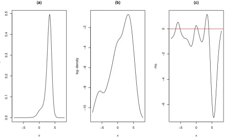
Figure 3: Plots of∇logπ(x) for the mixture example (left-hand column), and rates at which the continuous-time MCMC algorithm will switch from a negative to a positive velocity (right-hand column). For the latter plots we show rates for the canonical process (full lines), simple sub-sampling (dashed lines) and sub-sampling with control variates (dotted lines). The vertical dotted line shows the value of ˆx. Top row is for 150 data points, and the bottom row for 1,500 data points. Plots are restricted to areas of non-negligible posterior mass.

that for all these options for choosing λ+_{, the underlying stochastic process we are simulating is unchanged – it} is just the efficiency of the simulation algorithm that is affected.

If we compare the best implementation of continous-time MCMC with subsampling, using (13), to the best version of the canonical implementation we get that for the same accuracy the we would need just over 25 times as many iterations using subsampling. Each iteration would be quicker, however, as it would need access to just one, out of 150, data-points.

To see any substantial gains from using subsampling, we need to have a lower variance estimator of ∇logπ(x), using, for example, control variates (11). To implement this we need to upper bound our estimator of the rate. This is possible for this application as the absoluate value of the second derivate of logπi(x) is bounded. Assume

we can find a bound,C say, then we use a bounding rate

λ+(x) =|∇logπ(ˆx)|+nC|x−ˆx|. (14)

To implement the resulting algorithm we can again iterate the three steps given above. The only changes are that in step (1) we need to simulate the inter-event time from a point process with rate

˜

0 200 400 600 800 1000 −2 0 2 4 6 Time x_ t

0 10 20 30 40

0.0 0.2 0.4 0.6 0.8 1.0 Lag A CF

0 200 400 600 800 1000

−2 0 2 4 6 Time x_ t

0 10 20 30 40

0.0 0.2 0.4 0.6 0.8 1.0 Lag A CF

0 200 400 600 800 1000

−2 0 2 4 6 Time x_ t

0 10 20 30 40

0.0 0.2 0.4 0.6 0.8 1.0 Lag A CF

Figure 4: Trace plots (top row) and autocorrelation plots (bottom row) for three implementations of continuous-time MCMC: canonical process (left-hand column); simple sub-sampling (middle column) and subsampling with control variates (right-hand column). Auto correlation plots are values sampled every unit time-step from the continuous sample paths.

and in step (3) the probability of switching the velocity is

max{0,−v[∇logπ(ˆx) +n(∇logπI(xt+s)− ∇logπI(ˆx))]}

|∇logπ(ˆx)|+nC|xt+s−xˆ|

.

We can get some insight into the advantage of using control variates by calculating the expected rate of switching the velocity for the resulting algorithm and comparing with this rate for the other two implementations. This comparison is shown in Figure 3. We see a much lower rate of switching when we use control variates ifxis close to ˆx as compared to the simple sub-sampling approach. However the rate is actually larger if xis far from ˆx. Thus we see the importance of ˆxbeing close to the mode of the posterior. This picture is the same for both small,

n= 150, and larger,n= 1,500, data sets. However for larger data sets the posterior mass close to the posterior mode increases. As such the amount of time that algorithm will be in regions where using control variates is better will increase as we analyse larger data sets.

In Figure 4 we see output from the algorithm using control variates for n= 150. For such a small sample size, there appears to be little advantage in using control variates. The mixing in the tails is poor, due to the large variability of our esimators of the switching rate when x is not close to ˆx. Note that we can avoid this issue by using a hybrid scheme that estimates the rates using control variates when |x−xˆ| is small, and uses simple sub-sampling otherwise.

effective sample size (ESS), a standard measure of MCMC performance. Firstly note that for the canonical implementation, the amount of PDP time, t, we need to run the continuous-time MCMC for decreases with sample size. This is as described in the scaling limits discussed in Bierkens et al. (2016). The intuition is that for larger nthe posterior is more concentrated, and thus the underlying PDP process needs less time to explore the posterior. This property is also seen if we use subsampling with control variates. Without control variates, the actual switching rates of the underlying PDP increase quickly with n which slows down the mixing of the algorithm, and the amount of time, t, that we need to simulate the underlying PDP for does not change much withn.

The computational cost of each algorithm also depends on the number of iterations, that is the number of proposed event-times, of the algorithm per t; and the cost of each iteration. The former increases with n for all implementations. Overall, the number of iterations per ESS remains roughly constant when we use control variates. As the computation cost per iterations isO(1) we see evidence that this algorithm has a computational cost that does not increase withn. By comparison the number of iterations per ESS appears to increase roughly linearly with n if we use subsampling without control variates. (See Bouchard-Cˆot´e et al., 2017, for further empirical evidence of these scalings when we use sub-sampling with or without control variates).

For the canonical implementation, even using the best possible global bound on the event rate, we have the number of iterations per ESS remaining constant but the computational cost per iteration is O(n). Thus its overall computational cost will increase linearly with n. We see some evidence of these scalings if we look at the number of gradient evaluations associated with each observation that needs to be calculated per ESS. In situations where these gradients are expensive this would be a good proxy for the overall computational cost – and these results suggest using sub-sampling with control variates will be particularly useful for models where this is the case.

4

Continuous-Time Sequential Importance Sampling

We now consider continuous-time versions of sequential importance sampling. Such algorithms were first developed to solve the problem of simulating from a diffusion (see Oksendahl, 2007, for an introduction to diffusions). In this situation we have a diffusion process,Xt, defined as the solution to an SDE

dXt=b(Xt)dt+σ(Xt)dBt,

where b(x) is thed-dimensional drift, Bt isd dimensional Brownian motion, andσ(x) is a dby dmatrix that

defines the instantaneous variance of the process. We have an initial distribution p0(x) for the diffusion, and wish to sample from the distribution of the process at some future time or times. If we denote the density of this process at time t, by pt(x), then the challenge is to sample from pt(x) for diffusion processes where we cannot

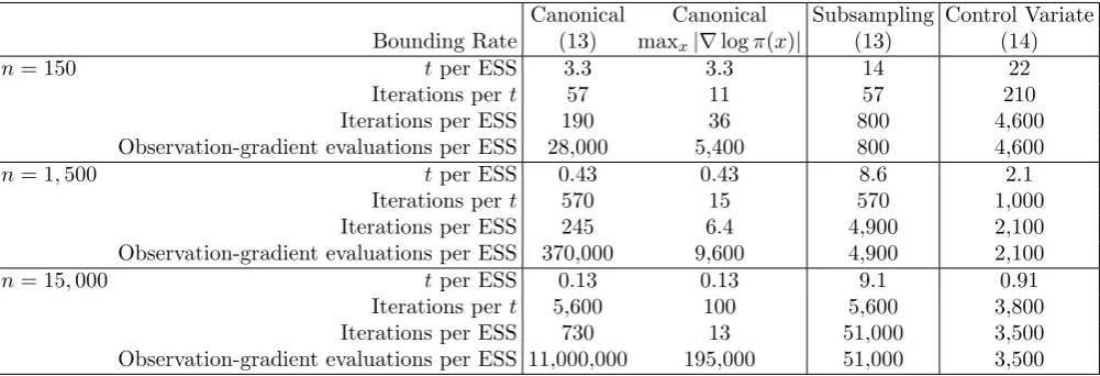
Canonical Canonical Subsampling Control Variate Bounding Rate (13) maxx|∇logπ(x)| (13) (14)

n= 150 t per ESS 3.3 3.3 14 22

Iterations pert 57 11 57 210

Iterations per ESS 190 36 800 4,600

Observation-gradient evaluations per ESS 28,000 5,400 800 4,600

n= 1,500 t per ESS 0.43 0.43 8.6 2.1

Iterations pert 570 15 570 1,000

Iterations per ESS 245 6.4 4,900 2,100

Observation-gradient evaluations per ESS 370,000 9,600 4,900 2,100

n= 15,000 t per ESS 0.13 0.13 9.1 0.91

Iterations pert 5,600 100 5,600 3,800

Iterations per ESS 730 13 51,000 3,500

Observation-gradient evaluations per ESS 11,000,000 195,000 51,000 3,500

Table 1: Comparison of different implementations of continuous-time MCMC: canonical, subsampling, and subsampling with control variates; and how they vary as sample size,n, increases. Both canonical and subsampling use a global bound on the event rate to simulate possible events, we give results for canonical using both (13) and maxx|∇logπ(x)|as this bound. We give estimates of both the stochastic process time-length,t, that the MCMC

algorithm needs to be run per effective sample size (ESS); and the average number of iterations (proposed event times) pert. The product of these is then the number of iterations needed per ESS. The subsampling and control variate versions require calculating the gradient associated with a single data point per iteration, whereas standard implementation requires nsuch evaluations; for each nwe also give the average number of such evaluations per ESS.

The Exact Algorithm (Beskos and Roberts, 2005; Beskos et al., 2006) and its variants (Beskos et al., 2008; Pollock et al., 2016b) have given a number of algorithms for simulating from such a diffusion process, but only under strong conditions on the drift and instantaneous variance. For example it is commonly required that σ(x) is constant, and that the drift can be written as the gradient of some potential function. Almost all uni-variate diffusion processes can be transformed to satisfy these requirements, but few multivariate diffusion processes can.

Whilst we do not know whatpt(x) is for anyt >0, we do know that it solves the Fokker-Planck equation for the

diffusion

∂pt(x)

∂t =−

d

∑

i=1

∂bi(x)pt(x)

∂xi

+1 2

d

∑

i=1

d

∑

j=1

∂2_Σ

ij(x)pt(x)

∂xixj

,

where Σ =σT_{σ. This motivates the following question: can we use our knowledge of the Fokker-Planck equation}

for the process of interest in order to develop a valid importance sampling algorithm to sample frompt(x)?

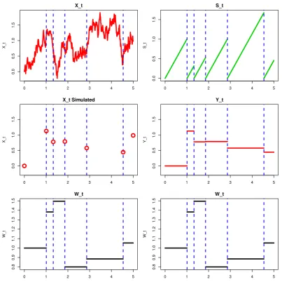
The continuous-time importance sampling (CIS) procedure of Fearnhead et al. (2016), which we describe below, will in fact enable us to do so. We will present it in a slightly more general form, in that we will use CIS to sample from a distributionpt(x) that is the solution to a partial differential equation

∂pt(x)

∂t =L

∗_p

t(x)