RANKING OF MAJOR STATES IN INDIA USING DATA ENVELOPMENT ANALYSIS (DEA) APPROACH
*Chandar
Department of Statistics, Loyola College (Autonomous), Chennai
ARTICLE INFO ABSTRACT
Data Envelopment Analysis (DEA), a non measure the relative
Units (or DMUs). The linear programming technique is employed to rank the 15 major states considered as DMUs in this study.
data structure and then the same linear programming (LP) technique is applied to the single reduced input and single reduced output. The states are ranked based on the result obtained by the analysis of reduced data and those rankings are compa
data. The results of this study showed that the ranking of States based on original data and the ranking of States based on reduced data vary considerably, which indicates that there may exists some inputs and/or outputs, though having less variance, can alter the rankings because of their high sensitivity, when processed using LP technique.
Copyright © 2014 Chandar and Edwin Prabakaran. This
unrestricted use, distribution, and reproduction in any medium, provided the original work is properly cited.
INTRODUCTION
Data Envelopment Analysis (DEA) is a nonparametric method used in operations research and economics to estimate the production frontiers. It is a linear programming method used for measuring the performance of homogeneous organizational units and is widely used in banking industries, where the bank branch will be the unit of measurement (Thanassoulis, 1999). DEA is not only used in banking, but also to analyze the relative efficiency of various sectors such as industrial firms, universities, military operations, banking, and healthcare or hospitals. In a study, it is used to evaluate the management of 60 Missouri Commercial Banks for the period f
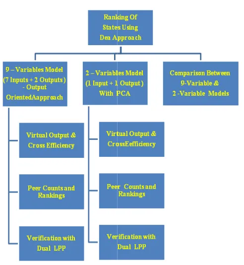
1990 (Yue, 1992). Jacobs (2000) has used three cost indices of the UK Department of Health to benchmark NHS Trusts. He compares the efficiency rankings from the cost indices with those obtained by the use of DEA and Stochastic Cost Frontier (SCF) Analysis. In this study, the DEA was applied to ra states within Indian Territory based on some inputs and outputs of Factor Sector taken from the Economic Appraisal of Tamil Nadu. The procedure for ranking of states using DEA approach is clearly described in the flow chart presented in the next section.
Flow Chart of Analysis
The procedure of ranking of states is clearly explained in the following flow chart:
*Correspoding author: Chandar, V.
Department of Statistics, Loyola College (Autonomous), Chennai Tamil Nadu, India.
ISSN: 0975-833X
Article History:
Received 15th August, 2014
Received in revised form
22nd September, 2014
Accepted 07th October, 2014
Published online 18th November,2014
Key words:
DEA, DMU, Cross-Efficiency, Relative-Efficiency, Peer, Ranking, PCA.
RESEARCH ARTICLE
RANKING OF MAJOR STATES IN INDIA USING DATA ENVELOPMENT ANALYSIS (DEA) APPROACH
Chandar, V. and Edwin Prabakaran, T.
Department of Statistics, Loyola College (Autonomous), Chennai - 600 034, Tamil Nadu, India
ABSTRACT
Data Envelopment Analysis (DEA), a non-parametric method, is used in this study to empirically measure the relative efficiency of major States in India, where the States are the Decision Making Units (or DMUs). The linear programming technique is employed to rank the 15 major states considered as DMUs in this study. Principal Component Analysis (PCA) is also applied to
data structure and then the same linear programming (LP) technique is applied to the single reduced input and single reduced output. The states are ranked based on the result obtained by the analysis of reduced data and those rankings are compared with the rankings obtained by the analysis of original data. The results of this study showed that the ranking of States based on original data and the ranking of States based on reduced data vary considerably, which indicates that there may exists e inputs and/or outputs, though having less variance, can alter the rankings because of their high sensitivity, when processed using LP technique.
This is an open access article distributed under the Creative Commons Attribution License, which permits unrestricted use, distribution, and reproduction in any medium, provided the original work is properly cited.
Data Envelopment Analysis (DEA) is a nonparametric method used in operations research and economics to estimate the production frontiers. It is a linear programming method used performance of homogeneous organizational units and is widely used in banking industries, where the bank branch will be the unit of measurement (Thanassoulis, 1999). DEA is not only used in banking, but also to analyze the ctors such as industrial firms, universities, military operations, banking, and healthcare or hospitals. In a study, it is used to evaluate the management of 60 Missouri Commercial Banks for the period from 1984 to three cost indices of the UK Department of Health to benchmark NHS Trusts. He compares the efficiency rankings from the cost indices with those obtained by the use of DEA and Stochastic Cost Frontier (SCF) Analysis. In this study, the DEA was applied to rank the states within Indian Territory based on some inputs and outputs of Factor Sector taken from the Economic Appraisal of Tamil Nadu. The procedure for ranking of states using DEA approach is clearly described in the flow chart presented in the next
The procedure of ranking of states is clearly explained in the
[image:1.595.312.558.421.688.2]Department of Statistics, Loyola College (Autonomous), Chennai - 600 034,
Figure 1. Flow Chart of Analysis
DEA Approach
Data Envelopment Analysis (DEA) is a nonparametric method used in operations research and economics to estimate the production frontiers. It is a linear programming (LP) model and used to empirically measure technica
Available online at http://www.journalcra.com
International Journal of Current Research
Vol. 6, Issue, 11, pp.9816-9822, November,2014
INTERNATIONAL
z
RANKING OF MAJOR STATES IN INDIA USING DATA ENVELOPMENT ANALYSIS (DEA) APPROACH
600 034, Tamil Nadu, India
parametric method, is used in this study to empirically efficiency of major States in India, where the States are the Decision Making Units (or DMUs). The linear programming technique is employed to rank the 15 major states Principal Component Analysis (PCA) is also applied to reduce the data structure and then the same linear programming (LP) technique is applied to the single reduced input and single reduced output. The states are ranked based on the result obtained by the analysis of red with the rankings obtained by the analysis of original data. The results of this study showed that the ranking of States based on original data and the ranking of States based on reduced data vary considerably, which indicates that there may exists e inputs and/or outputs, though having less variance, can alter the rankings because of their high
Creative Commons Attribution License, which permits
Flow Chart of Analysis
Data Envelopment Analysis (DEA) is a nonparametric method used in operations research and economics to estimate the production frontiers. It is a linear programming (LP) model and used to empirically measure technical efficiency of decision
making units (or DMUs). Although the concept of DEA is mostly applied in the field of production theory in economics, the tools of DEA are also used for benchmarking in operations management, where a set of measures is selected to improve the performance of manufacturing and service operations (Cooper et al., 2002).
In particular, DEA is a multi-factor productivity analysis model used to measure the relative efficiencies of a homogenous set of decision making units (DMUs). When there are multiple input and output factors, the efficiency score can be defined as follows:
Inputs
of
Sum
Weighted
Outputs
of
Sum
Weighted
Efficiency
Assuming that there are n DMUs with n1 inputs and n2 outputs,
the relative efficiency score of a test DMU 'k' (i.e., with kth DMU as the reference DMU) is obtained by solving the following LP model proposed by Cooper et al.(2002):
2 1 n j j k j kV
m
Z
Maximize
Subject to the constraints
1
1 1
n j j k j kU
l
n
i
for
U
l
V
m
n j j i j k n j j i jk
0
,
1
,
2
,
3
,
.
.
.
,
1 2 1 1
whereUij denoted the j th
Input of the ith DMU
Vij is the jth Output of the ith DMU
mkj is the weights given to jth output of kth DMU (for j = 1 to
2
n
)lkj is the weights given to jth input of kth DMU (for j = 1 to
n
1)By solving the above Linear Programming Problem (LPP), the optimal weights can be obtained for a kth reference DMU (i.e.,
j k
m
andl
kj). Using these optimal weights of the kth reference DMU, the Cross Efficiency of each of the other DMUs can be calculated as below:Cross Efficiency (CE)
If there are n DMU’s with
n
1 inputs andn
2 outputs, then theCross Efficiency of the
s
th DMU (Doyle and Green, 1994), denoted by CE(s, k), is given by
1 2 1 1)
,
(
n i i s i k n i i s i kU
l
V
m
k
s
CE
, where k is the reference DMU; s k; and s = 1, 2, 3, . . . , n
mk,i and lk,i are the optimal weights derived for the kth
reference DMU for the corresponding outputs and inputs respectively
Vs,i = ith output of the sth DMU and Us,i = ith input of the
sth DMU
If the Cross Efficiency, CE(s, k) of the sth DMU is equal to 1, then the corresponding sth DMU is considered as a Peer to the kth reference DMU (a better terminology may be “Dominating DMU”).
The Dual of the above LPP can be utilized to cross check the Peers obtained by the corresponding cross efficiency scores. Let kth DMU be the reference DMU. Then the dual of the above LPP is given as follows:
Minimize Z* =
Subject to the constraints
1 1
,
.
.
.
,
2
,
1
,
j
n
U
U
p
kjn
i
j i i
k
2 1,
.
.
.
,
2
,
1
,
j
n
V
V
p
kjn
i
j i i
k
j i all forpij 0,
0 ,(Ui,j = jth input of the ith DMU & Vi,j = jth output of the ith
DMU; n = number of DMUs)
The concept of cross efficiency and peers can be cross checked with the help of the above dual i.e., if a DMU turns out to be a Peer for a particular reference DMU, then the DMU in the corresponding dual will a positive weight.
The above LPP which maximizes the virtual output and its corresponding dual are known as Output Oriented Approach. In a similar way, we can have an Input Oriented Approach, in which the virtual input can be minimized, fixing the virtual output at a fixed level. The results arrived by both the approaches (i.e., Input oriented and Output oriented LPPs) will lead to the same set of rankings.
Data Reduction using PCA Technique
Principal Component Analysis (PCA) is a statistical technique used to linearly transform an original set of variables into a considerably smaller set of uncorrelated variables that represents majority of the information in the original set of variables. Principal Components are linear combinations of random or statistical variables which have special properties in terms of variance (Dunteman, 1989). The DMU theory is explorative in nature and the ranking of the DMUs is very much depends upon the Inputs and Outputs that are included in the model. Initially to begin with, a certain judicious choice of Inputs and Outputs are considered. Here, normally not all Inputs and Outputs considered are independent and thereby a multiple-colinearity exists in the Input-Output structure. To avoid this type of redundancy, which affects the efficiency of the ranking process, the ‘Principal Component Analysis’ is employed. Thus using PCA technique, the number of Inputs and number of Outputs are reduced to their first few Principal Components. After reduction if the structure and the final ranking of the DMUs remain unaltered then one can conclude that certain Inputs and Outputs are redundant and they can be dropped based on the weights of their Principal Components. On the other hand, if there is a change either in the structure of the Cross Efficiency matrix or in its final ranking then one can conclude that the reduction of Inputs and Outputs is not possible and the original set of Inputs and Outputs are to be maintained.
Dataset used in this study
In this study 15 major States within Indian Territory are considered and those States are as follows:
1. Andhra Pradesh 2. Assam
3. Bihar 4. Gujarat 5. Haryana 6. Karnataka 7. Kerala
8. Madhya Pradesh 9. Maharashtra 10. Orissa 11. Punjab 12. Rajasthan 13. Uttar Pradesh 14. West Bengal 15. Tamil Nadu.
For each State, 7 Inputs and 2 Outputs are considered, which are listed below:
The 7 Inputs are
1. The number of industries 2. Fixed Capital
3. Productive Capital 4. Number of workers 5. Wages paid to workers 6. Number of Employees 7. Total Emoluments
The 2 Outputs are
1. Value of Output 2. Net value added
The above inputs and Outputs are taken from the “Annual Survey of Industries (ASI)” – Survey results (Factory Sector) in Government of India – Ministry of Statistics and Programme Implementation (MOSPI). (http://mospi.nic.in/mospinew/ upload/asi/asi_table3_9900.htm)
Data Analysis
Linear programming technique is exploited to rank or order the decision-making units (DMU). In our study each of the 15 major states is considered as a DMU. The process of ranking utilizes certain selected inputs (say n1-inputs) and outputs (say
n2-outputs). The n1 inputs are reduced to a single virtual input
by taking the linear combination of the n1 inputs, the weights
being selected using a Linear Programming Problem (LPP) which maximizes the virtual output. This virtual output is again a linear combination of the corresponding n2 outputs of a
selected DMU, which is referred to as “REFERENCE DMU”. That is, the DMU for which the weights are derived is called the ‘Reference DMU’ and its efficiency is called ‘Self Efficiency’.
The inputs and outputs of particular units are used to derive an efficiency measure, which involves the ratio of virtual output to virtual input. The virtual input and virtual output are the weighted linear combination of the n1-Inputs and n2-Outputs respectively of a unit. The weights are selected in such a way that the ratio of virtual output to virtual input is maximized for a particular unit over the space which gives reasonable importance for other comparable decision making units i.e., the unit virtual output is maximized over the space governed by the performance of other comparable DMUs. If the weights derived for a particular Reference DMU are applied to other DMUs, the resulting efficiency of other DMUs is called ‘Cross Efficiency’. For a particular DMU, if the Cross Efficiency corresponding to some other State is 1 (one) then that State is considered as a Peer (a better terminology may be “Dominating DMU”) with respect to the corresponding Reference DMU. Thus the frequency of Peers of a particular State, which is denoted by “Peer Count”, serves as a measure of “Relative Efficiency”, which in turn will help us to rank the States.
If tie occurs among the Peer Counts then the Self Efficiency of each State can be utilized to rank the States.
Ranking of States using Virtual Efficiency
Calculation of Self-Efficiency: To begin with, the State “Andhra Pradesh” has been considered as a reference DMU and the optimal weights for the inputs and outputs are obtained using Linear Programming Technique. Then using these optimal weights, the self-efficiency of the State “Andhra Pradesh” has been calculated. The LPP for the State “Andhra Pradesh” has been formulated using the notations given in Section 2 and is shown in Appendix. By solving the LPP constructed for the State “Andhra Pradesh”, the Self Efficiency of Andhra Pradesh was obtained as Maximum Z = 0.7311222525. By proceeding this way, we obtained the optimal weight for inputs and outputs and the self-efficiency scores for all the remaining 14 States and are shown in Table A1.
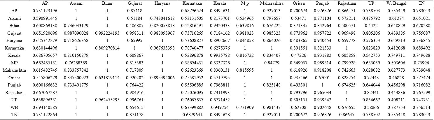
Calculation of Cross-Efficiency: Using the optimal weights of Andhra Pradesh, the derivation of Cross Efficiency of the State ‘Kerala’ was obtained using the formula shown in Section 2. Using the values of Input and Output variables of ‘Kerala’, the Cross-Efficiency of Kerala with Andhra Pradesh as reference DMU was calculated to be 0.8494631. In the same way, the Cross efficiency of Assam with Andhra Pradesh as Reference DMU was found to be exactly 1. Similarly, by taking each State as reference DMU, the Cross Efficiency scores of other States have been calculated in the same way and are shown in Table A2.
Calculation of Peers: For each Reference State, the corresponding other States with Cross Efficiency values as one are considered as Peers of the Reference State. Peers can be considered as performing in an efficient manner with respect to the Reference State (Reference DMU). From the Cross Efficiency values given in Table A2, we obtained the Peers for each Reference State and are shown in Table A3.
Calculation of Peer Counts: Using Table A3, we count the number of times a particular State is regarded as a Peer for other States. A State which acts as Peer for more States has ‘Relative best performance’ and hence “Peer Counts” serve as an indicator of its relative efficiency. The Table A4 shows the Peer Counts for each Reference State.
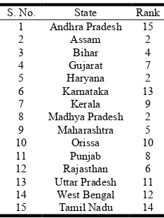
[image:4.595.104.221.609.764.2]States and their Ranks: Based on the peer counts and the self-efficiency scores, the states have been ranked and the corresponding result is shown in Table 6.1.
Table 6.1. States and their Ranks based on their Peer Counts and Self Efficiency using Original Data
S. No. State Rank
1 Andhra Pradesh 15
2 Assam 2
3 Bihar 4
4 Gujarat 7
5 Haryana 2
6 Karnataka 13
7 Kerala 9
8 Madhya Pradesh 2
9 Maharashtra 5
10 Orissa 10
11 Punjab 8
12 Rajasthan 6
13 Uttar Pradesh 11
14 West Bengal 12
15 Tamil Nadu 14
The Peers of a State derived by using the Cross Efficiency can be verified by solving the Dual LPP of that State. In the corresponding dual problem, Peers alone will have non-zero solution. That is, the states for which the solution is non-zero will be the Peers for the Reference DMU. This dual property is verified in the case of Andhra Pradesh by solving the dual LPP of Andhra Pradesh.
The dual LPP corresponding to Andhra Pradesh was formulated and solved, and the corresponding result showed that the Self Efficiency of Andhra Pradesh is 0.7311222525 (i.e., Minimum Z*), which coincides with Maximum Z obtained by solving the corresponding Primal LPP. For the Primal problem, the Peers given in Table A3 for the State “Andhra Pradesh” are Assam, Bihar, Haryana and Madhya Pradesh. For the corresponding dual problem, the solution is non-zero only for the states Assam, Bihar, Haryana and Madhya Pradesh, while the solution becomes zero for the other States. This property provides an alternative approach for finding the peers of a State (DMU). This clearly shows that the ranking of states obtained by solving Primal LPP will the same as the rankings obtained by solving the corresponding Dual problem.
Data Reduction using PCA Technique
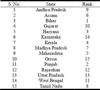
The Principal Component Analysis is a technique of data reduction. That is, if there are ‘n’ records each with ‘m’ variables then, the PCA reduces the ‘m’ variables into ‘k’ (k<n) linear combinations of the original ‘m’ variables. These linearly transformed variables retain a considerable variation of the data (n x m - values). In Section 5, the states were ranked using their 7 Inputs and 2 Outputs. In this Section, the 7 Inputs and 2 Outputs are reduced to Single Input and Single Output using Principal Component Technique. The results of this PCA showed that in both Input and Output reductions, the 1st Principal Component takes into account a considerable amount of variation. Therefore, our study is restricted to the 1st Principal Component in both the cases - i.e., Input Reduction and Output Reduction. Using the First Principal Component, we obtained the Single Reduced Input and Single Reduced Output for all the 15 States, and this reduced data is shown in Table A5. Then the 15 States were ranked based on these reduced Input and Reduced Output by using the same analysis used in Section 5 and the corresponding result showed that the Self Efficiency of Andhra Pradesh is Minimum Z* = 0.5724932105, which coincides with Maximum Z obtained by solving the corresponding Primal LPP. For the Primal problem, the Peers for the State Andhra Pradesh were found to be ‘Bihar’. For the corresponding Dual problem, the solution is non-zero only for the State Bihar, while the solution is zero for the other States. The ranking of 15 states based on this reduced data is shown in Table A6.
Conclusion
Analysis. This implies that there may exists some Inputs and/or Outputs, though having less variance, can alter the rankings because of their high sensitivity, when processed through LPP optimization. It is suggested from the results of this study that instead of reducing the data dimension using Principal Component Technique (which has been established as a failure), other measures of influence can be devised for each Input and Output variables and there by the data volume can be reduced with the same relative rankings.
REFERENCES
Cooper, W.W., Seiford, L.M., and Tone, K. 2002. Data Envelopment Analysis: A Comprehensive Text with Models, Applications, References and DEA-Solver Software. Kluwer Academic Publishers, Dordrecht. Doyle, J and Green, R. 1994. Efficiency and cross efficiency in
DEA: derivations, meanings and uses. Journal of the Operational Research Society, 45(5): 567-578.
Dunteman, G.H. 1989. Principal Components Analysis. SAGE Publications, Beverly Hills, Calif.
Jacobs, R. 2000. Alternative Methods to Examine Hospital Efficiency: Data Envelopment Analysis and Stochastic Frontier Analysis, Health Care Management Science, 4(2): 103-16.
Principal Characteristics (Factory Sector) by Major States in India for the year 1999-00. Retrieved from: http://mospi.nic.in/mospi_new/upload/asi/asi_table3_9900. htm
Thanassoulis, E. 1999. Data Envelopment Analysis and its Use in Banking. Interfaces, Vol.29, No.3, pp. 1-13.
Yue, P 1992. “Data Envelopment Analysis and Commercial Bank Performance: A Primer with Applications to Missouri Banks.” Federal Reserve Bank of St. Louis Economic Review, 74(1): 31-45.
Appendix
The LPP for the State “Andhra Pradesh” has been formulated and is presented below:
Max Z = 5849398 m1,1 + 911042 m1,2
Subject to the constraints
13164 l1,1 + 2712037 l1,2 + 3214547 l1,3 + 770522 l1,4 + 214354 l1,5 + 910356 l1,6 + 337197 l1,7 = 1
-13164 l1,1 - 2712037 l1,2 - 3214547 l1,3 - 770522 l1,4 - 214354 l1,5 - 910356 l1,6 - 337197 l1,7 + 5849398 m1,1 +911042 m1,2 ≤ 0
…………. …………. …………. ………….
- 6373 l1,1 - 1740738 l1,2 – 1797696 l1,3 – 462666l1,4 – 258194 l1,5 - 588968 l1,6 - 377712 l1,7 + 3485892 m1,1 + 573679 m1,2 ≤ 0
- 20249 l1,1 - 3750517 l1,2 – 4722285 l1,3 – 888350 l1,4 – 312910 l1,5 - 1103970 l1,6 - 515876 l1,7 + 9459777 m1,1 + 1479535 m1,2 ≤ 0
where m1,j ≥ 0 , j = 1, 2 and l1,j ≥ 0, j = 1, 2, 3, 4, 5, 6, 7
The solution of the above LPP is given below: The optimal weights for inputs are
l11 = 0.0000136645
l12 = 0
l13 = 0.0000000956
l14 = 0
l15 = 0
l16 = 0
and l17 = 0.0000015203
The optimal weights for outputs are m11 = 0.0000000719 and m12 = 0.0000003406. The Self Efficiency of Andhra Pradesh is
Maximum Z = 0.7311222525.
Proceeding as above, we obtained the optimal weight for inputs and outputs and self-efficiency scores for all the remaining 14 States and are presented in Table A1.
Table A1. Self Efficiency of the States
S.No. State
Optimal Weights
Self Efficiency
Inputs Outputs
IP1 IP2 IP3 IP4 IP5 IP6 IP7 OP1 OP2
1 Assam 0 0 0.0000025821 0 0 0 0.0000023092 0 0.0000058894 1
2 Bihar 0 0 0.0000044804 0 0 0 0 0.0000014992 0 1
3 Gujarat 0 0.00000002 0.00000002 0.00000024 0.0000008 0 0.00000074 0.00000002 0.00000039 0.9583112118
4 Haryana 0 0 0.0000004081 0 0 0.0000008704 0 0.0000002249 0 1
5 Karnataka 0.0000251081 0 0.0000000207 0.0000000536 0.0000030229 0 0.0000008225 0 0.0000009433 0.7874051830
6 Kerala 0.0000460608 0 0.0000008703 0 0 0 0 0.0000003996 0 0.9935795518
7 Madhya Pradesh 0 0 0.0000002081 0 0 0.0000006919 0.0000020872 0.0000002268 0 1
8 Maharashtra 0 0 0.0000000786 0 0 0.0000002423 0 0.0000000259 0.0000001532 1
9 Orissa 0.0002693074 0 0 0 0 0 0.0000068008 0 0.0000034978 0.9354655385
10 Punjab 0 0.0000003269 0 0.0000010836 0 0 0.0000024600 0.0000002617 0 0.9991956927
11 Rajastan 0 0.0000000548 0.0000000742 0 0.0000032392 0.0000008075 0.0000024732 0.0000000757 0.0000014550 1
12 Uttar Pradesh 0 0.0000000491 0 0.0000003620 0.0000023068 0 0.0000007967 0.0000000180 0.0000007083 0.8346662850
13 West Bengal 0.0000330604 0 0.0000004391 0 0 0 0 0.0000000923 0.0000008121 0.7877515204
14 T_N 0.0000090333 0 0.0000000632 0 0 0 0.0000010051 0.0000000476 0.0000002252 0.7830422600
Table A2. Cross Efficiency of the States
AP Assam Bihar Gujarat Haryana Karnataka Kerala M p Maharashtra Orissa Punjab Rajasthan UP W. Bengal TN
AP 0.731123196 1 1 0.87118 1 0.68796524 0.8494631 1 0.927013 0.700674 0.976876 0.866471 0.738503 0.535449 0.783043
Assam 0.590991445 1 1 0.51184 0.743041618 0.53131505 0.8173701 0.524965 0.797657 0.53471 0.771104 0.572211 0.475792 0.61274 0.651021
Bihar 0.608869138 0.736033179 1 0.486887 0.820053818 0.42816491 0.9320333 0.639816 0.676222 0.371335 0.842964 0.500571 0.4422 0.648829 0.670288
Gujarat 0.651920696 0.987090028 0.992224193 0.958311 0.988093967 0.73716265 0.7184162 0.981023 0.985323 0.773962 0.957722 0.969498 0.805206 0.439385 0.755087
Haryana 0.625342279 0.718626358 1 0.65995 1 0.53608827 0.8902667 0.844858 0.864026 0.483865 0.940454 0.659778 0.576353 0.629213 0.736845
Karnataka 0.630144496 1 0.809270814 1 0.967633398 0.78740477 0.6275376 1 1 0.891551 0.821333 1 0.823829 0.412068 0.689492
Kerala 0.686705657 0.810150879 1 0.609867 1 0.52896878 0.9935788 0.816722 0.834407 0.47226 0.931882 0.605858 0.542753 0.749711 0.749688
MP 0.662485151 0.76268369 1 0.815383 1 0.58694451 0.8337326 1 0.84779 0.549057 0.989814 0.799928 0.685059 0.503606 0.75996
Maharashtra 0.615482745 0.833757842 1 0.717809 1 0.62623369 0.8360131 0.815595 1 0.618926 0.918208 0.742663 0.628082 0.627773 0.739048
Orissa 0.545806279 0.847500923 0.621819114 0.920202 0.895494006 0.75581952 0.5719795 1 1 0.935466 0.67001 0.828254 0.72443 0.46828 0.577474
Punjab 0.600166632 0.733491779 1 0.764422 1 0.55506885 0.7968811 1 0.825148 0.493301 1 0.674625 0.644044 0.456298 0.716082
Rajasthan 0.667067287 1 1 0.984916 1 0.75026095 0.7311993 1 1 0.793796 0.965034 1 0.82341 0.443836 0.767599
UP 0.638896351 1 0.962455295 0.996761 1 0.76067857 0.6771452 1 1 0.805151 0.939842 1 0.834667 0.408211 0.743731
WB 0.693140585 1 1 0.654615 1 0.63399882 0.949754 0.771909 0.981437 0.62708 0.902648 0.676655 0.58866 0.787753 0.756514
[image:6.842.51.795.294.500.2]Table A3. Peers for Reference States
S. No. Reference state Peers
1 Andhra Pradesh Assam, Bihar, Haryana, M_P
2 Assam Assam
3 Bihar Bihar
4 Gujarat Assam, Gujarat
5 Haryana Haryana
6 Karnataka Assam, M_P, Maharashtra, Rajasthan
7 Kerala Bihar, Haryana
8 Madhya Pradesh M_P
9 Maharashtra Maharashtra
10 Orissa M_P, Maharashtra
11 Punjab Bihar, Haryana, M_P
12 Rajasthan Rajasthan
13 Uttar Pradesh Assam, Haryana, M_P, Maharashtra ,Rajasthan
14 West Bengal Assam, Bihar, Haryana
15 Tamil Nadu Assam, Bihar, Haryana, M_P
Table A4. Peer Counts for Reference States
S. No. Reference state Peers count
1 Andhra Pradesh 0
2 Assam 7
3 Bihar 6
4 Gujarat 1
5 Haryana 7
6 Karnataka 0
7 Kerala 0
8 Madhya Pradesh 7
9 Maharashtra 4
10 Orissa 0
11 Punjab 0
12 Rajasthan 3
13 Uttar Pradesh 0
14 West Bengal 0
[image:7.595.324.538.75.229.2]15 Tamil Nadu 0
Table A5. Reduced Input and Reduced Output for 15 States
S. No. States Reduced Input Reduced Output
1 Andhra Pradesh 7694723.704 6746919.12
2 Assam 824755.138 945494.222
3 Bihar 505513.952 774239.418
4 Gujarat 15976738.12 13755128.61
5 Haryana 3718005.385 5085595.426
6 Karnataka 6906419.221 5075018.622
7 Kerala 2186168.775 2843577.448
8 Madhya Pradesh 4404503.924 4962666.776
9 Maharashtra 18508573.58 21548839.95
10 Orissa 2241536.138 1447203.792
11 Punjab 3188585.678 4368195.102
12 Rajasthan 4329014.996 3520415.06
13 Uttar Pradesh 9289799.136 7113394.7
14 West Bengal 4934390.252 4051451.858
15 Tamil Nadu 10648112 10917433.38
Table A6. States and their Ranks based on their Peer Counts and Self Efficiency Using Reduced Data
S. No. State Rank
1 Andhra Pradesh 9
2 Assam 6
3 Bihar 1
4 Gujarat 10
5 Haryana 3
6 Karnataka 14
7 Kerala 4
8 Madhya Pradesh 7
9 Maharashtra 5
10 Orissa 15
11 Punjab 2
12 Rajasthan 12
13 Uttar Pradesh 13
14 West Bengal 11
15 Tamil Nadu 8