Evaluate the Investment Efficiency by Using Data Envelopment Analysis: The Case of China

(1)

Evaluate the Investment Efficiency by Using Data

Envelopment Analysis: The Case of China

Hualun Zhang, Wei Song, Xiaobao Peng, Xiaoyan Song School of Public Affairs, University of Science and Technology of China, Hefei, China

Email: [email protected]

Received March 2, 2012; revised April 7, 2012; accepted April 18, 2012

ABSTRACT

Although investment is regarded as a key force of China’s economic growth, little study has been done to measure China’s investment efficiency. The present paper applies the data envelopment analysis (DEA) to Chinese provincial panel data from the year 2003 to 2008 for measuring the investment efficiencies and identifying their trends of Chinese 30 provinces and autonomous regions. A cross-efficient DEA model with considering benevolent formulation is used for providing accurate efficiency scores and completely ranking. The empirical results suggest that the differences of investment efficiency in different regions are distinct but tending to diminish year by year, and the investment efficiencies in some provinces are significantly correlated to their investment rates to the national total investment.

Keywords: Aggregate Investment; Efficiency; Data Envelopment Analysis (DEA)

1. Introduction

Chinese economy development has gained the great su- ccess in the past two decades that attracts worldwide attention. Many researchers confirmed importance of the aggregate investment in the Chinese economic growth and performance see [1-3], which has taken up about 30% of gross domestic product (GDP) see [4,5]. The China’s growth pattern is also similarly considered as the investment-growth model in [6]. More and more researchers start to study the investment and investment efficiency, because the importance of investment in Chinese economic growth is widely acknowledged.

In [1,2] admit that aggregate investment plays a important role in China’s phenomenal economic growth after estimating China’s aggregate economy by consumption function, investment function and production function, respectively. [7] suggests that fixed-capital investment is the most important determinant of China’s economic growth, and China follows an investment-driven expansion path in the 1980-1990s. [8] apply the exogeneity framework to investigate empirically the relationship between investment and growth in China. They find that there is a robust and significant relation of capital formation on output growth, suggesting that the fixed investment is a key determinant of China’s economic growth. Since investment has been regarded as an important force of China’s economic growth, In [4] propose a fixed capital formation to explore and explain the de-

terminants of China’s aggregate investment based on a panel data set of 28 provinces and autonomous regions. The empirical results they obtained show the existence of a homogenous equilibrium correction mechanism in China’s aggregate investment process and imply the su- ggestion that it is important to introduce favorable investment incentives in the central and west regions for balancing the economic growth. In [5] divide the aggregate investment in China into business sector investment and government direct investment and separately assess each of them by composing a suitable investment model. Their results suggest that the business sector investment is largely determined by market forces while the government direct investment is found to bear strong planned features. In [9] utilize macroeconometric models to measure the validity of the belief that the Chinese economy still follows largely the investment-led growth paradigm growth. By using the post-1990 annual data, they con- firm the relation between investment and economy growth, and suggest that the problem of overinvestment still exists in China.

(2)

[image:2.595.58.287.111.444.2]

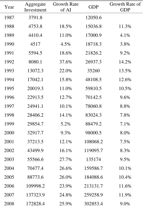
Table 1. China’s growth rates of aggregate investment and GDP.

Year Aggregate Investment

Growth Rate of AI GDP

Growth Rate of GDP 1987 3791.8 12050.6 1988 4753.8 18.5% 15036.8 11.3% 1989 4410.4 11.0% 17000.9 4.1% 1990 4517 4.5% 18718.3 3.8% 1991 5594.5 18.6% 21826.2 9.2% 1992 8080.1 37.6% 26937.3 14.2% 1993 13072.3 22.0% 35260 13.5% 1994 17042.1 15.8% 48108.5 12.6% 1995 20019.3 11.0% 59810.5 10.5% 1996 22913.5 12.7% 70142.5 9.6% 1997 24941.1 10.1% 78060.8 8.8% 1998 28406.2 14.1% 83024.3 7.8% 1999 29854.7 5.2% 88479.2 7.1% 2000 32917.7 9.3% 98000.5 8.0% 2001 37213.5 12.1% 108068.2 7.5% 2002 43499.9 16.1% 119095.7 8.3% 2003 55566.6 27.7% 135174 9.5% 2004 70477.4 26.6% 159586.7 10.1% 2005 88773.6 26.0% 184088.6 10.4% 2006 109998.2 23.9% 213131.7 11.6% 2007 137323.9 24.8% 259258.9 11.9% 2008 172828.4 25.9% 302853.4 9.0%

decentralisation imposes a variety of interregional barri- ers to trade and causes the inefficient in resource allocation. By analyzing the variation of total factor productivity and investment returns during the 1990s, In [12] assert that China’s allocative efficiency is significantly enhanced by the continuous sectoral shift of labor force. [10] maintain that the phenomenon of over-investment and inefficient investment still exists in China by composing a model that based on the standard capital factor input demand theory with associate measures of allocative inefficiency and technical inefficiency.

Although many studies have been done to verify the importance of aggregate investment to China’s growth and the existence of China’s over-investment, there has little research on measuring the China’s investment efficiency detailed from intuitionistic angle. This study seeks to evaluate the efficiency of the aggregate investment of 30 provinces and autonomous regions in China for the year 2003 to 2008 by using a model with relate concepts called cross-efficiency evaluation method. Then, we set out to explore and explain the changing trend of the performances during the six years and provide some man- age suggestions for the corresponding decision makers

based on the empirical results. The rest of the paper is organised as follows. Section 2 introduces the mathe- matical programming model used in the study. Applica- tion and empirical results are presented in Section 3, while the final section concludes the paper.

2. Methodology

Data envelopment analysis (DEA), proposed by [13], has become a popular efficiency evaluation tool and its de- rivative models have been widely used in many fields to measure the relative efficiency of peer decision making units (DMUs) on the basis of their multiple inputs and outputs. [14] extend DEA to the cross-efficiency evaluation method for identifying the best performing DMUs and ranking them by using cross-efficiency scores that obtained by all of the DMUs. The main idea of cross- efficiency evaluation is to use DEA in a peer evaluation mode, rather than in a self-evaluation mode.

Adopting the conventional nomenclature of DEA, as- sume that there are n DMUs that are to be evaluated in terms of m inputs and s outputs. We denote the ith input an rth output for DMUj (j = 1, ···, n) as ij

t

x (i = 1, ···, m) and rj (r = 1, ···, s) at each time period t, t = 1, ···, T. The efficiency scores of each DMUd (d = 1, ···, n) based on the traditional input-oriented DEA model proposed by [13] can be obtained by the following linear programming model (1) as:

t y





1 1 1 1 Max ,

. . 0, 1, , ,

1,

0, 1, 2, , ,

0, 1, 2, , . s

t t t

r rd d k k

r

m s

t t

i ij r rj

i r m i id i i r

y x y

t x y j n

x i m r s                    



   s (1)



,



t t t d xk yk 

, , , , ,

is the optimal result of the above model, which shows the performance of DMUd based on a traditional CCR model at the period t.

1d md 1d sd

 __ _ _ _





are the optimal weights obtained by the model (1). Then the cross efficiency of any DMUj (j = 1, ···, n) at period t, using the weight has cho- sen by DMUd in model (1) can be computed as:

1

, , , 1, , .

s t rd rj

t t t r

dj k k m t id ij i

y

E x y d j n

k

t



k

y

… … … … … …

n



t



k

y 2 , t t n k E x 1 , t t n k

E x 3



,



d k k exactly equal to the optimal result t xt y



,



t t t

E x y

 . Then, we average each the columns of cross efficiency matrix (CEM) in Table 1 to get a mean cross efficiency measure for each DMU. So, the cross-efficiency score of DMUk (k = 1, ···, n) at period t should be obtained by averaging all dk k k (d = 1, ···, n), namely









1

,

t t t

dk k k

E x y

, , , 1

,

n

t t t

k k k

d E x y

n 





(k = 1, ···, n). In fact, the weights 1d, ,md 1d sd

 

 

1

, , ,

d d sd

 

1d, , m

obtained by maximizing DMUd’ simple efficiency scores may not unique, that possibly reduces the perceived usefulness of cross-efficiency. One remedy suggested is to introduce a secondary objective function to resolve the ambiguity see [14,15]. Following their studies, we conclude a benevolent secondary formulation, which could be utilized to maximize the other DMU’s cross-efficiencies based on all the possible weights     

1 1

, 1, , ,

0, t r rd l n y       



,



t t t E x y

 

obtained by model (1):









1 1 1 1 Max , . 0 1, ,

0, 1, 2, , , 0, 1, 2, , .

s t t t

dj k k r rj

r

m s

t t

i il r rl

i r

m i ij r

m s

t t t t

i id dd k k

i r

E x y y

s t x y

x

x E x y

i m r s                   



   (3)

The optimal value dj k k of model (2), denot- ing the maximum efficiency scores of DMUj based on DMUd at period t, could be used to determine the ulti- mate cross efficiency of each DMUk at period t:





3. Application

3.1. Data Description

There are a great number of input and output variables, whether tangible and intangible, that can describe the influencing factors and results of investment. However, China’s economic growth depends very much on the rapid expansion of manufacturing sector see [12]. Taking the factors that have been suggested in the existing li- terature and data available into consideration, we choose three input variables: Fixed-asset investment at provincial level (X1); Net fixed asset of industry at provincial level (X2); Number of employee of industry at provincial level (X3), while two major economic indicators are selected: Gross Domestic Product (GDP) at the provincial level (Y1); and the Value-added of industry at provincial level (Y2). In this paper, all the input and output variables are selected from Chinese Statistical Yearbook, and six years from 2003 to 2008 are considered.

3.2. Efficiency Analysis

The CCR efficiency score of the 30 different provinces in China was firstly assessed using the traditional model (1). From Table 3, we can find that there are 7 efficient provinces in 2003, 9 in 2004, 9 in 2005, 11 in 2006, 11 in 2007 and 10 in 2008. Four east region provinces (namely, Beijin, Shanghai, Guangdong and Hainan) and one mid region province (Heilongjiang) keep efficient in all the five years considered, while 17 provinces poorly perform during 2003 to 2008. Besides, we can also conclude from the above table that the performance of east region is better than the mid and west region because of more efficient provinces and higher average efficiency score. However, this CCR efficiency score might not good enough. Firstly, it is calculated by using the weight selected itself, which heavily weights few favorable measures and completely ignores other inputs and outputs in order to maximize its own DEA efficiency. Secondly, we can not completely rank the performance of the 30 provinces based on these CCR efficiency scores. Finally, for the good-performance provinces (such as Beijing, whose efficiency score keeping 1 during the six years), CCR efficiency scores can not reflect the performance changes over the six years.

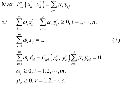
Table 4 reports the cross-efficiency scores of the 30

provinces during 2003 to 2008 by utilizing the model (2). As indicated in Table 2, no province is complete efficient measured by the cross-efficiency DEA model. To further analyze the cross-efficiency results, we classify all the 30 provinces and autonomous regions into three groups according to the economic region they belong to and compare the average efficiency scores of each group in the six years, see Figure 1. Note that the efficiency scores of the east region are higher than the mid, while



t_k



,k 1, , .n

  

1

1 n

t t t t t

k k k dj k

d

E x , y E x , y

n





[image:3.595.93.291.509.647.2]

(4)

[image:4.595.58.539.101.551.2]

Table 3. CCR efficiency scores of different provinces.

Regions Province 2003 2004 2005 2006 2007 2008 BJ 1 1 1 1 1 1 TJ 0.892 0.977 0.985 1 1 1 HB 0.900 0.914 0.902 0.895 0.912 0.896 LN 0.833 0.724 0.745 0.743 0.765 0.730 SH 1 1 1 1 1 1

JS 0.999 1 0.883 0.907 0.879 0.833 ZJ 0.927 0.972 0.751 0.744 0.783 0.816 FJ 1.000 0.961 0.957 0.952 0.923 0.973

SD 0.997 1 1 1 1 1

GD 1 1 1 1 1 1 East regions

HAN 1 1 1 1 1 1 SX 0.750 0.750 0.741 0.725 0.753 0.714 NMG 0.746 0.749 0.900 0.919 1.000 1.000 JL 0.848 0.843 0.783 0.799 0.897 0.822 HLJ 1 1 1 1 1 1

AH 0.909 0.870 0.890 0.885 0.857 0.767 JX 0.844 0.909 0.963 0.964 0.909 0.708 HN 0.946 0.937 0.932 0.967 1 1 HUB 0.771 0.766 0.824 0.834 0.824 0.772 Mid regions

HUN 1 0.968 1 1 1 1

GX 1 0.997 1 1 1 0.957

CQ 0.785 0.846 0.845 0.863 0.825 0.819 SC 0.788 0.797 0.857 0.848 0.879 0.878 GZ 0.666 0.679 0.688 0.724 0.737 0.745 YN 0.951 1 0.967 1 0.949 0.926 SHX 0.697 0.694 0.700 0.778 0.930 0.807

GS 0.666 0.700 0.719 0.797 0.783 0.734 QH 0.580 0.685 0.750 0.771 0.860 0.857 NX 0.502 0.532 0.586 0.579 0.644 0.651 West regions

XJ 0.921 1 1 1 1 1

Table 4. Cross-efficiency scores of provinces during 2003 to 2008.

Regions Province 2003 2004 2005 2006 2007 2008 BJ 0.827 0.859 0.834 0.808 0.818 0.834 TJ 0.718 0.768 0.767 0.869 0.868 0.867 HB 0.778 0.791 0.765 0.772 0.775 0.759 LN 0.698 0.632 0.639 0.636 0.653 0.632 SH 0.858 0.841 0.792 0.788 0.816 0.830 JS 0.783 0.786 0.736 0.748 0.725 0.662 ZJ 0.692 0.695 0.619 0.605 0.607 0.629 FJ 0.863 0.802 0.758 0.725 0.672 0.696 SD 0.757 0.768 0.811 0.790 0.797 0.806 GD 0.899 0.879 0.816 0.785 0.749 0.727 East regions

[image:4.595.55.537.570.736.2]

(5)

Continued

SX 0.600 0.613 0.574 0.540 0.572 0.585 NMG 0.648 0.617 0.662 0.682 0.733 0.693 JL 0.750 0.742 0.677 0.664 0.710 0.666 HLJ 0.888 0.888 0.916 0.912 0.871 0.887 AH 0.767 0.711 0.728 0.724 0.680 0.617 JX 0.665 0.649 0.688 0.746 0.713 0.577 HN 0.785 0.768 0.759 0.797 0.868 0.868 HUB 0.657 0.635 0.648 0.629 0.680 0.656 Mid regions

HUN 0.812 0.779 0.816 0.852 0.842 0.799 GX 0.810 0.763 0.785 0.829 0.799 0.740 CQ 0.639 0.605 0.608 0.666 0.636 0.615 SC 0.674 0.673 0.710 0.726 0.752 0.737 GZ 0.579 0.583 0.578 0.612 0.615 0.628 YN 0.843 0.831 0.775 0.793 0.763 0.767 SHX 0.607 0.597 0.617 0.667 0.765 0.685 GS 0.561 0.580 0.570 0.591 0.631 0.629 QH 0.424 0.458 0.469 0.482 0.533 0.544 NX 0.442 0.459 0.495 0.499 0.558 0.552 West regions

XJ 0.635 0.673 0.731 0.773 0.765 0.847

Average efficiency scores of different regions in China

0.50 0.55 0.60 0.65 0.70 0.75 0.80 0.85

1 2 3 4 5 6

Year

E

ff

ici

en

cy

sco

res

[image:5.595.59.538.98.370.2]

East Mid West

Figure 1. Average efficiency scores of different regions in China.

the efficiency values of mid regions are also higher than the western. Also, more details should be found:  The changes of efficiency scores of east provinces are

very small which express a trend downward.

 The wave of efficiency scores of mid regions are significant.

 The improvement of west provinces are more pro- nounced.

Besides, the phenomenon of convergence is illustrat- ing in figure 1 too during 2003 to 2008, which might be due to the Chinese central planning to promote the regional productivity equality see [16]. However, that phenomenon might also caused by the over-investing in the east region and infrastructure construction enhancing in

the mid and west regions. By comparing the average ef-ficiency scores in different years, we find that the regional efficiency gap evidently decreased from 2003 to 2008, which might indicate that the investment allocation and productivity in different regions across the country are becoming reasonable and equal.

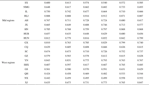
Table 5 reports the complete ranking of different pro-

[image:5.595.103.501.393.539.2]

(6)

[image:6.595.63.539.102.500.2]

Table 5. Ranking of cross-efficiency scores of provinces during 2003 to 2008.

Regions Province 2003 2004 2005 2006 2007 2008

BJ 7 3 2 5 6 5

TJ 16 12 9 2 3 3

HB 12 8 10 12 10 11

LN 17 22 22 23 23 21

SH 4 4 6 9 7 6

JS 11 9 14 13 17 19

ZJ 18 17 23 26 27 22

FJ 3 7 13 16 22 15

SD 14 11 5 8 9 8

GD 1 2 4 10 15 14

East regions

HAN 5 6 11 18 5 7

SX 26 24 27 28 28 27

NMG 22 23 20 19 16 16

JL 15 15 19 22 19 18

HLJ 2 1 1 1 1 1

AH 13 16 16 17 21 25

JX 20 20 18 14 18 28

HN 10 13 12 6 2 2

HUB 21 21 21 24 20 20

Mid regions

HUN 8 10 3 3 4 9

GX 9 14 7 4 8 12

CQ 23 25 25 21 24 26

SC 19 19 17 15 14 13

GZ 27 27 26 25 26 24

YN 6 5 8 7 13 10

SHX 25 26 24 20 12 17

GS 28 28 28 27 25 23

QH 30 30 30 30 30 30

NX 29 29 29 29 29 29

West regions

XJ 24 18 15 11 11 4

Sichuan and Xinjiang, had increasingly improved their performance order, while two provinces (namely, Anhui and Guangdong) have shown a continuous decreasing trend. Take XinJiang for example, its ranking order in- creased from the 24th to 4th during the period 2003-2008. The increase could probably be attributed to the work done by the managers during these six years in improving the efficiency of using the investment. On the other hand, as the ranking order decreased from 1st to 14th during the six years, Guangdong province is an example of the typical provinces which are significant slippage. The decision makers need to do more work to reverse the dis- advantageous situation by improving the efficiency of resource use.

3.3. Correlational Analysis between the Efficiency Scores and Investment

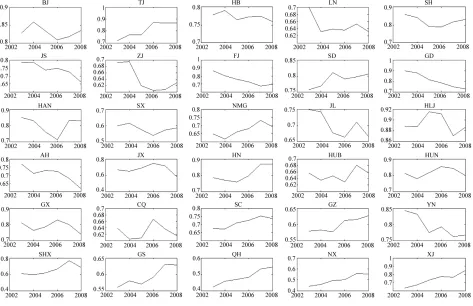
The above Figure 2 shows the trend of the cross-effi-

ciency scores of all the 30 provinces during 2003 to 2008. Some provinces express an upward tendency (such as Tianjin, Gansu, Qinghai, Ningxia and Xinjiang), while some others show a downward tendency (such as Jiangsu, Fujian, Guangdong and Anhui). Besides, note that, most of the provinces in west region keep their efficiency as- cendant in these years.

Figure 3 gives the curves of ratio of provincial invest-

(7)

[image:7.595.64.537.88.394.2] [image:7.595.62.540.227.695.2]

Figure 2. Cross-efficiency scores of provinces during 2003 to 2008.

(8)

[image:8.595.58.539.99.230.2]

Table 6. Results of Spearman correlation between efficiency score and investment ratio.

East region BJ TJ HB LN SH JS ZJ FJ SD GD HAN Spearman Correlation 0.143 –0.429 0.714 –0.486 0.486 0.886 0.543 –0.771 0.086 1.000 0.257 Sig. (2-tailed) 0.787 0.397 0.111 0.329 0.329 0.019 0.266 0.072 0.872 0 0.623 Middle region SX NMG JL HLJ AH JX HN HUB HUN

Spearman Correlation –0.771 0.943 –0.657 –0.600 –0.829 –0.257 0.771 0.371 –0.143 Sig. (2-tailed) 0.072 0.005 0.156 0.208 0.042 0.623 0.072 0.468 0.787

West region GX CQ SC GZ YN SHX GS QH NX XJ Spearman Correlation –0.314 0.086 0.314 –0.829 –0.771 0.771 0.600 –1.000 –0.943 –0.943

Sig. (2-tailed) 0.544 0.872 0.544 0.042 0.072 0.072 0.208 0 0.005 0.005

more investment shift to middle region.

It is seen from Table 6 that the efficiency scores of eight provinces (Jiangsu, Guangdong, Neimenggu, Anhui, Guizhou, Qinghai, Ningxia and Xinjiang) have significant correlation1 with the investment ratios. Then, these eight provinces can be divided into four categories. The two east region provinces Jiangsu and Guangdong belong to the first category, whose efficiency scores decline with the investment ratios falling. However, on the contrary, the four west region provinces (Guizhou, Qinghai, Ning- xia and Xinjiang) improve their performance as the investment ratios decreasing and compose the second category. Lastly, two middle region provinces, Neimenggu and Anhui, are respectively called the third and fourth category because of their different response to the increasing investment ratio. The efficiency score of Nei- menggu grow with the increasing of investment ratio, while the performance of Anhui gets worse significantly as investment raise sharply.

4. Conclusions

This paper applies a cross-efficiency DEA model to measure the investment efficiency of 30 provinces in China in order to provide a detailed regional analysis of Chinese investment inefficiency. Three inputs (Fixed- asset investment, Net fixed asset of industry and Number of employee of industry) and two outputs (GDP and Value-added of industry) and provincial-panel data for the period 2003-2008 are considered in this study. A number of interesting results with important implications are found:

Based on the empirical results, there are very significant differences between the three economic regions in China: the east region is the best performance while the west region is the worst. This is very understandable because of the disparities in the infrastructure. Better investment environment is provided by the east region through years of accumulation, while the mid and west regions do not have a requirement to make full use of the

investment.

On the other hand, the assimilation appears in nation- wide: the difference of the performances between the three regions is diminishing by comparing the trend of efficiencies during 2003-2008. That phenomenon is not only an expression of the improvement of allocative efficiency but also the inevitable result that economy grows. Moreover, more work need to be done to narrow the gap between different regions in the further.

Investment is driving force for some east province such as Jiangsu and Guangdong that is expressed as the significant positive correlation between the decrease of investment and efficiency, while the over-investment does exist in some west provinces such as Guizhou, Qinghai, Ningxia and Xinjiang because of the significant negative correlation between the investment decreasing and performance improving.

REFERENCES

[1] G. C. Chow, “A Model of Chinese National Income De-termination,” Journal of Political Economy, Vol. 93, No. 4, 1985, pp. 782-791. doi:10.1086/261330

[2] G. C. Chow, “Capital Formation and Economic-Growth in China,” Quarterly Journal of Economics, Vol. 108, No. 3, 1993, pp. 809-867. doi:10.2307/2118409

[3] L. X. Sun, “Estimating Investment Functions Based on Cointegration: The Case of China,” Journal of Compara- tive Economics, Vol. 26, No. 1, 1998, pp. 175-191. doi:10.1006/jcec.1997.1501

[4] H. Song, Z. Liu and P. Jiang, “Analysing the Determi- nants of China’s Aggregate Investment in the Reform Pe-riod,” China Economic Review, Vol. 12, No. 2-3, 2001, pp. 227-242. doi:10.1016/S1043-951X(01)00052-9 [5] X. He and D. Qin, “Aggregate Investment in People’s

Republic of China: Some Empirical Evidence,” Asian Development Review, Vol. 21, 2004, pp. 99-117.

[6] J. Zhang, “Capital Formation, Industrialization and Eco- nomic Growth,” Economic Research Journal, Vol. 7, 2002, pp. 3-13 (in Chinese).

[7] Q. Yu, “Capital Investment, International Trade and Economic Growth in China: Evidence in the 1980-90s,”

(9)

China Economic Review, Vol. 9, No. 1, 1998, pp. 73-84. doi:10.1016/S1043-951X(99)80005-4

[8] A. C. C. Kwan, Y. Wu and J. Zhang, “Fixed Investment and Economic Growth in China,” Economics of Planning, Vol. 32, No. 1, 1999, pp. 67-79.

doi:10.1023/A:1003424418042

[9] D. Qin, M. A. Gagas, P. Quising and X. He, “How Much Does Investment Drive Economic Growth in China?” Journal of Policy Modeling, Vol. 28, No. 7, 2006, pp. 751-774. doi:10.1016/j.jpolmod.2006.02.004

[10] D. Qin and H. Song, “Sources of Investment Inefficiency: The Case of Fixed-Asset Investment in China,” Journal of Development Economics, Vol. 90, No. 1, 2009, pp. 74- 145. doi:10.1016/j.jdeveco.2008.06.001

[11] A. Young, “The Razor’s Edge Distortions and Incre-mental Reform in the People’s Republic of China,” The Quarterly Journal of Economics, Vol. 115, No. 4, 2000, pp. 1091-1136. doi:10.1162/003355300555024

[12] J. Zhang, “Investment, Investment Efficiency, and

Eco-nomic Growth in China,” Journal of Asian Economics, Vol. 14, No. 5, 2003, pp. 713-734.

doi:10.1016/j.asieco.2003.10.004

[13] A. Charnes, W. W. Cooper and E. Rhodes, “Measuring the Efficiency of Decision Making Units,” European Jour- nal of Operational Research, Vol. 3, No. 4, 1970, pp. 429- 444. doi:10.1016/0377-2217(79)90229-7

[14] T. R. Sexton, R. H. Silkman and A. J. Hogan, “Data En-velopment Analysis: Critique and Extensions,” In: R. H. Silkman, Ed., Measuring Efficiency: An Assessment of Data Envelopment Analysis, Jossey-Bass, San Francisco, 1986, pp. 73-105.

[15] J. Doyle and R. Green, “Efficiency and Cross Efficiency in DEA: Derivations, Meanings and the Uses,” Journal of the Operational Research Society, Vol. 45, 1994, pp. 567- 578.