Novel methods for distributed acoustic sensing data

acoustic sensing data

Rebecca Elizabeth Wilson, M.Math, M.Res

Submitted for the degree of Doctor of

Philosophy at Lancaster University.

In this thesis, we propose novel methods for analysing nonstationary, multivariate time series, focusing in particular on the problems of classification and imputation within this context. Many existing methods for time series classification are static, in that they assign the entire series to one class and do not allow for temporal depen-dence with the signal. In the first part of this thesis, we propose a computationally efficient extension of an existing dynamic classification method to the online setting. Dependence within the series is captured by adopting the multivariate locally sta-tionary wavelet (mvLSW) framework and the signal is classified at each time point into one of a number of known classes. We apply the method to multivariate acoustic sensing data in order to detect anomalous regions and evaluate the results against alternative methods in the literature. The second part of this thesis considers im-putation in multivariate locally stationary time series containing missing values. We first introduce a method for estimating the local wavelet spectral matrix that can be used in the presence of missingness. We then propose a novel method for imputing missing values that uses the local auto and cross-covariance functions of a mvLSW process to perform one step-ahead forecasting and backcasting. The performance of

Firstly, I would like to thank my supervisors Idris Eckley and Matt Nunes for all the advice and guidance that they have provided throughout this project.

I am grateful for the financial support provided by the EPSRC and Shell. I would also like to thank my industrial supervisor Tim Park for the helpful discussions and insights into the project and the data provided.

I would like to thank the staff and students at the STOR-i Doctoral Training Centre for providing a stimulating and enjoyable research environment.

Finally, I would like to thank my family for their encouragement and support over the years, this would not have been possible without you.

I declare that the work in this thesis has been done by myself and has not been submitted elsewhere for the award of any other degree.

Chapter 3 has been accepted for publication as Wilson, R. E., Eckley, I. A., Nunes, M. A. and Park, T. (2018). Dynamic detection of anomalous regions within distributed acoustic sensing data streams using locally stationary wavelet time series. Data Mining and Knowledge Discovery.

Chapter 4: Wilson, R. E., Eckley, I. A., Nunes, M. A. and Park, T. (2018). A wavelet-based approach for imputation in highdimensional series. In preparation.

Chapter 5: Wilson, R. E., Grose, D., Eckley, I. A., Nunes, M. A. and Park, T. (2018). mvLSWimpute: An R package for imputation in multivariate locally stationary time series. In preparation for submission to the R Journal.

Rebecca Elizabeth Wilson

Word count: 44424

Abstract I

Acknowledgements III

Declaration IV

List of Figures XII

List of Tables XVI

List of Algorithms XVII

1 Introduction 1

2 Literature Review 4

2.1 Introduction to wavelets and their transforms . . . 5

2.1.1 Fourier Analysis . . . 5

2.1.2 Multiresolution Analysis (MRA) . . . 7

2.1.3 Wavelet Families . . . 10

2.1.4 Discrete Wavelet Transform (DWT) . . . 12

2.1.5 Non-decimated Wavelet Transform (NDWT) . . . 16

2.2 Time Series Analysis . . . 20

2.2.1 Stationary time series modelling . . . 22

2.2.2 Nonstationary time series modelling . . . 25

2.3 Wavelets in Time series . . . 28

2.3.1 Locally Stationary Wavelet model . . . 29

2.3.2 Multivariate Locally Stationary Wavelet framework . . . 33

2.4 Classification of nonstationary time series . . . 38

2.4.1 Static classification . . . 39

2.4.2 Dynamic classification . . . 41

3 Dynamic detection of anomalous regions within distributed acoustic sensing data streams using locally stationary wavelet time series 44 3.1 Introduction . . . 44

3.2 Online dynamic classification of multivariate series . . . 50

3.2.1 Edge Effects . . . 52

3.3 Synthetic Data Examples . . . 57

3.4 Case Study . . . 71

3.5 Concluding remarks . . . 77

3.6 Online nondecimated wavelet transforms . . . 78

3.7 Comparison of computational cost of online classification methods . . 80

4.2 Background . . . 86

4.2.1 Forecasting univariate locally stationary time series . . . 86

4.2.2 Forecasting multivariate locally stationary wavelet processes . 87 4.3 Imputation for multivariate locally stationary wavelet processes . . . 89

4.3.1 Spectral Estimation . . . 91

4.3.2 Forecasting . . . 93

4.3.3 Backcasting . . . 94

4.4 Simulated performance of mvLSWimpute . . . 95

4.4.1 Competitor methods . . . 100

4.4.2 Evaluation measures . . . 102

4.5 Case study . . . 109

4.6 Concluding remarks . . . 113

4.7 Bursts of missingness . . . 114

4.8 Simulated performance of mvLSWimpute - additional tables . . . 115

5 mvLSWimpute: An R package for imputation in multivariate locally stationary time series 120 5.1 Introduction . . . 120

5.2 mvLSWimpute approach . . . 123

5.2.1 Spectral Estimation . . . 124

5.2.2 Forecasting . . . 132

5.2.3 Backcasting . . . 135

5.4 Summary . . . 143

6 Conclusions and Discussion of Future Work 145 A onlineDC: R package 149 A.1 The onlineDC package functions . . . 149

A.1.1 Simulating multivariate normal training data . . . 150

A.1.2 Obtaining information from the training data . . . 151

A.1.3 Applying Dynamic Classification method . . . 153

A.1.4 Applying Dynamic Classification with a moving window . . . 155

A.1.5 Combining probabilities . . . 158

2.1.1 Example of the Gibbs effect . . . 6 2.1.2 Daubechies Extremal Phase mother wavelets forN = 1,3 and 6. . . . 11 2.1.3 Example of the lack of translation-invariance of the DWT; (a) shows

the original data whilst (b) shows the data rotated by a unit shift. Figures (c) and (d) depict the Haar DWT for the original and shifted data respectively. . . 17 2.1.4 Example of the translation-invariance of the NDWT; (a) shows the

original data whilst (b) shows the data rotated by a unit shift. Figures (c) and (d) depict the Haar NDWT for the original and shifted data respectively. . . 19 2.3.1 Example showing the effect of correcting the raw wavelet periodograms. 33

3.1.1 Time series plots of DAS amplitude at four different well depths over the same time period: (a) original series; (b) detrended series. The highlighted regions in (a) indicate three examples of striping. . . 47

3.1.2 Hidden time-varying coherence structure of the DAS series in Figure 3.1.1 at selected wavelet scales (resolutions): (a) coherence between series 1 and 2; (b): coherence between series 3 and 4. . . 48 3.2.1 Realisation of a two class time-varying vector autoregressive moving

average process, where a change in class takes place at time 300. . . 54 3.2.2 Probability of belonging to each class for various windows of data, the

true class change at time 300 is marked in red. . . 55 3.2.3 Average probabilities and class membership of the series over time. . 56 3.3.1 Example realisations of generating processes for the different scenarios

used in the simulation study. (a) Short segments of length 100 between class changes; (b) Alternating long/short segments of length 300 and 100 between changes; (c) Long segments of length 300 between changes. 61 3.4.1 Q-Q plots for the original and transformed coherence between channels

2 and 3 for the first window of the data. . . 74 3.4.2 Classification results obtained from applying online dynamic

classifi-cation, Sequential HMM and Embedded HMM approaches to acoustic sensing data, areas of the signal for which a change in class is detected are shown in red. . . 76 3.7.1 Comparison of computational cost of the classification methods

4.4.1 Example realisations of generating processes for the different scenarios used in the simulation study. (a), (c) Slowly evolving dependence, class changes at time 150 and 300; (b) Rapidly changing dependence structure, class changes at time 100, 200, 300 and 400; (d) Stationary signal, no changes in the generating coefficient matrices of the process. 97 4.5.1 Time series plots of the CO2 concentration for three sensors over the

same time period: (a) original series; (b) detrended series. . . 110 4.5.2 Imputation results obtained from applying mvLSWimpute-fb, mtsdi

and VAR-fb approaches to CO2 data, imputed values are shown in red. 111 4.5.3 Imputation results for August 5 only, imputed values are shown in red. 112 4.7.1 Example time series containing bursts of missingness. . . 114

5.2.1 Example realisation of the process. (a) True signal; (b) Signal after missingness has been induced. . . 127 5.2.2 Average spectra across 100 replications of the slowly evolving mvLSW

process; True spectral values shown in black, spectral values generated using mvEWS shown in red and the spectral estimates for the missing data are shown in blue. . . 130 5.2.3 Average spectra across 100 replications of the time varying vector

au-toregressive process; spectral values generated using mvEWS shown in red and the spectral estimates for the missing data are shown in blue. 131 5.2.4 True series and signal after applying the mvLSWimpute forecasting

5.2.5 True series and signal after applying mvLSWimpute method. . . 137 5.3.1 Time series of four European financial indices. . . 138 5.3.2 Time series of four European financial indices, for each series 10% of

values are missing. . . 140 5.3.3 European Financial Indices time series after imputing missing values

using mvLSWimpute. . . 141 5.3.4 European Financial Indices time series after imputing missing values

using mtsdi. . . 142 5.3.5 Sum of the absolute differences between the imputed time series and

the truth. (a) mvLSWimpute; (b) mtsdi. . . 143

A.1.1Probability estimates from different windows at time 200. . . 158 A.1.2The result of using the different display options to plot the onlineDC

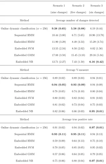
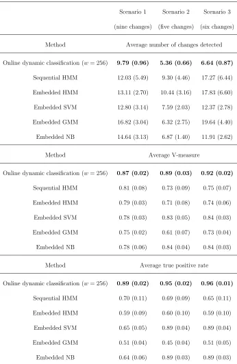
3.3.1 Performance of classification procedures over 100 replications of mul-tivariate Gaussian series for different scenarios of class changes, using the evaluation measures described in the text. Numbers in brackets represent the standard deviation of estimation errors. Bold numbers indicate best result. . . 67 3.3.2 Performance of classification procedures over 100 replications of vector

moving average series for different scenarios of class changes, using the evaluation measures described in the text. Numbers in brackets represent the standard deviation of estimation errors. Bold numbers indicate best result. . . 68 3.3.3 Performance of classification procedures over 100 replications of

vec-tor auvec-toregressive series for different scenarios of class changes, using the evaluation measures described in the text. Numbers in brackets represent the standard deviation of estimation errors. Bold numbers indicate best result. . . 70

3.3.4 Performance of online dynamic classification algorithm with differing window lengths over 100 replications of multivariate Gaussian series for different scenarios of class changes, using the evaluation measures described in the text. Numbers in brackets represent the standard deviation of estimation errors. Bold numbers indicate best result. . . 72

4.4.1 Performance of the imputation methods over 100 replications of mvLSW process with slowly evolving dependence for different missingness sce-narios occurring simultaneously across all channels, using the evalua-tion measures described in the text. Numbers in brackets represent the standard deviation of estimation errors. Bold numbers indicate best result. . . 104 4.4.2 Performance of the imputation methods over 100 replications of vector

4.4.3 Performance of the imputation methods over 100 replications of vector autoregressive series with slowly evolving dependence structure for dif-ferent missingness scenarios occurring simultaneously across all chan-nels, using the evaluation measures described in the text. Numbers in brackets represent the standard deviation of estimation errors. Bold numbers indicate best result. . . 106 4.4.4 Performance of the imputation methods over 100 replications of

sta-tionary vector moving average series for different missingness scenarios occurring simultaneously across all channels, using the evaluation mea-sures described in the text. Numbers in brackets represent the standard deviation of estimation errors. Bold numbers indicate best result. . . 107 4.8.1 Performance of the imputation methods over 100 replications of mvLSW

process with slowly evolving dependence for different missingness sce-narios occurring across one channel, using the evaluation measures de-scribed in the text. Numbers in brackets represent the standard devi-ation of estimdevi-ation errors. Bold numbers indicate best result. . . 116 4.8.2 Performance of the imputation methods over 100 replications of vector

4.8.3 Performance of the imputation methods over 100 replications of vec-tor auvec-toregressive series with slowly evolving dependence structure for different missingness scenarios occurring across one channel, using the evaluation measures described in the text. Numbers in brackets repre-sent the standard deviation of estimation errors. Bold numbers indicate best result. . . 118 4.8.4 Performance of the imputation methods over 100 replications of

sta-tionary vector moving average series for different missingness scenarios occurring across one channel, using the evaluation measures described in the text. Numbers in brackets represent the standard deviation of estimation errors. Bold numbers indicate best result. . . 119

1 Online dynamic classification: Finding the average probability that a multivariate signal belongs to a particular class over time. . . 53 2 mvLSWimpute: Steps carried out in one iteration of the method. . . 90

Introduction

In recent years, there has been a rapid increase in high-resolution sensors collecting large amounts of data over short periods of time. One example is the high frequency acoustic sensing data generated within the oil and gas sector, often sampled at a rate of 10kHz per second across a range of depths within an oil well. This data collection results in large multivariate time series that can be difficult to model and analyse for a number of reasons. For example, it can be hard to capture complex inter-variable relationships or the series may be nonstationary in nature. In particular, the second-order structure may change over time. Wavelets, a form of localised basis functions, offer one possible approach to solving this problem. Their localisation in both time and scale allows for more efficient modelling of data containing locally changing behaviour or discontinuities (Dahlhaus, 2012).

Within the existing wavelet literature, Nason et al. (2000) introduced the locally stationary wavelet processes as a way of accurately modelling univariate time series exhibiting smoothly varying second-order structure. In the multivariate setting,

elling individual channels of the series using the LSW framework can be deficient as relationships between variables are not taken into account. To this end, Park et al. (2014) developed the multivariate locally stationary wavelet framework which accu-rately captures the dependence structure between components of a multivariate time series. A review of the properties of wavelets and their transforms is provided in Chapter 2, along with a discussion of time series modelling and the wavelet-based approaches discussed above.

One of the main challenges associated with industrial sensing technology is that the recordings can be corrupted with periods of anomalous behaviour which have a negative impact on any secondary analysis such as forecasting or performance mod-elling. In Chapter 3, we introduce a computationally efficient extension of the dynamic classification method of Park et al. (2018) to the online setting. This permits real-time classification of a multivariate real-time series with changing class membership over time. We conclude the chapter by assessing the performance of the proposed classifier using simulated time series and demonstrating how it can be used to detect anoma-lous regions within multivariate acoustic sensing data. Details of the software that implements the online dynamic classification method can be found in Appendix A.

that can be used to estimate missing values within a multivariate locally stationary time series. We extend the wavelet forecasting approach of Fryzlewicz and Ombao (2009) to the multivariate setting and combine this with a backcasting step to improve accuracy. We again assess the performance of the proposed method against competi-tor methods through simulated examples and a dataset arising from a Carbon Capture and Storage facility. The software that implements the imputation method is avail-able in the R package mvLSWimpute, details of the package and a demonstration of it’s functionality can be found in Chapter 5.

Literature Review

This chapter reviews the literature on wavelets and time series modelling that are required for the work presented in the other chapters of this thesis. The first part of the chapter provides an introduction to wavelets and an overview of some popular transforms. We begin by briefly summarising key aspects of Fourier analysis, pointing out shortcomings of the approach and scenarios in which it will provide poor decom-position results. Wavelets are introduced in Section 2.1.2 through the concept of a multiresolution analysis and some popular wavelet families are summarised in Sec-tion 2.1.3. A variety of wavelet transforms are discussed in SecSec-tions 2.1.4 and 2.1.5 including the discrete wavelet transform, the non-decimated wavelet transform and wavelet packet transforms.

In the second part of the chapter, we review some approaches for modelling time series. Section 2.2.1 covers methods for modelling stationary time series in both the time and frequency domain. Some approaches for modelling nonstationary time series through locally stationary representations are discussed in Section 2.2.2

ing Locally Stationary Fourier processes (Dahlhaus, 1997) and the Smooth Localized Exponential model (Ombao et al., 2002). An alternative method for modelling non-stationary time series using wavelets as the basis functions is then discussed. The (univariate) Locally Stationary Wavelet processes (Nason et al., 2000) are described in detail in Section 2.3.1 before the Multivariate Locally Stationary Wavelet frame-work (Park et al., 2014) is discussed in Section 2.3.2. In the final part of the chapter, various approaches for the classification of nonstationary time series are discussed including the SLEX-based method of Huang et al. (2004) and the wavelet-based ap-proaches of Fryzlewicz and Ombao (2009), Krzemieniewska et al. (2014) and Park et al. (2018).

2.1

Introduction to wavelets and their transforms

2.1.1

Fourier Analysis

Within classical Fourier analysis, a periodic square integrable functionf ∈L2_{([−π, π]),} can be represented in terms of the Fourier basis{exp(inx)}∞

n=−∞in the following way

f(x) =

∞

X

−∞

cnexp(inx), (2.1.1)

where the Fourier coefficients are computed by

cm = (2π)−1

Z π

−π

f(x)exp(−imx)dx. (2.1.2)

One of the main drawbacks associated with Fourier series decomposition is that it cannot efficiently deal with discontinuities in a signal due to the nature of the basis functions {cos(nx),sin(nx)}n∈Z. Specifically, these functions are smooth and

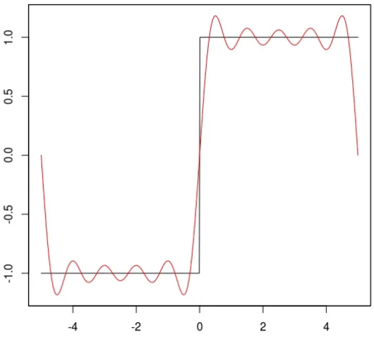
have infinite support meaning that every basis sine and cosine function will interact with a discontinuity which will influence the coefficients of the Fourier transform. An example of this can be seen in Figure 2.1.1, the Fourier series representation of the function near the discontinuities is poor and Gibbs effects can clearly be seen.

Figure 2.1.1: Example of the Gibbs effect

of Fourier theory, see Walker (1986) or Percival and Walden (2006).

In order to efficiently model functions containing discontinuities, alternative basis functions are required that capture local features more accurately. Specifically, we require basis functions that are compactly supported. Wavelet basis functions possess this quality, as well as allowing for time-scale decomposition of a signal. For this reason, wavelets are often seen as a desirable alternative to Fourier approaches in situations where discontinuities or nonstationarity are present in a signal. In the next section, we introduce wavelets through the idea of a multiresolution analysis before discussing some of the commonly used wavelet basis functions.

2.1.2

Multiresolution Analysis (MRA)

A multiresolution analysis (MRA), first introduced in Meyer (1986) and Mallat (1989a), is a sequence of closed subspaces{Vj}_j∈ZinL2(R) such that the following containment holds

. . .⊂V−2 ⊂V−1 ⊂V0 ⊂V1 ⊂V2 ⊂. . . (2.1.3) In order to be considered a MRA, this sequence of closed subspaces must also satisfy some additional conditions given by

1. [ j∈Z

Vj =L2(R).

2. \ j∈Z

Vj ={0}.

3. f(2jx)∈Vj ⇐⇒ f(x)∈V0.

expressed as a linear combination of translated copies of φ(x). As such, the set

{φ(x−k)}_k∈

Z is an orthonormal basis of V0.

The scaling function φ(x) is also known as the father wavelet. As a consequence of Conditions 3 and 4, we can see that the set

{φj,k(x) = 2

j

2φ(2jx−k)} k∈Z

is a basis ofVj for some fixed j.

A wavelet basis is characterised by two functions, the father wavelet as defined above and a mother wavelet function. If we have subspaces that satisfy the conditions for a MRA then we can define the mother wavelet. First we must define the subspace Wj which is the orthogonal complement of Vj in Vj+1. In other words,

Vj+1 =Vj⊕Wj.

Due to this relation, we can write any function g(x) ∈ Vj+1 uniquely as a linear combination of elements of Vj and Wj. I.e. g(x) = vj(x) +wj(x) where vj(x) ∈ Vj and wj(x)∈Wj.

If we have a sequence of subspaces that satisfy the conditions for a MRA then there exists an orthonormal basis for _L2(_R) given by

{ψj,k(x) = 2

j

2ψ(2jx−k)} j,k∈Z,

such that {2j2ψ(2jx−k)}

k∈_Z is an orthonormal basis of Wj for fixed j. As a conse-quence of this we can define the mother wavelet, ψ(x) =ψ0,0(x).

definition of MRA, specifically relation (2.1.3), we obtain the containment V0 ⊂ V1. As a consequence of this, we can conclude thatφ(x)∈V1. Therefore we can represent φ(x) as a linear combination of functions from V1, which has an orthonormal basis given by {φ1,k(x) =

√

2φ(2x−k)}_k∈

Z. From this we can obtain the dilation equation

φ(x) =X k∈Z

hkφ1,k(x) =

X

k∈Z hk

√

2φ(2x−k) (2.1.4)

where H = {hk}k∈_Z is the low-pass filter. In a similar way we can obtain the

corre-sponding dilation equation forψ(x)

ψ(x) =X k∈_Z

gkψ1,k(x) =

X

k∈_Z

gk

√

2ψ(2x−k) (2.1.5)

whereG ={gk}k∈Z is the high-pass filter.

In addition, we can use MRA to show that the following links exist between the father and mother wavelets

ψ(x) = X k∈Z

gk

√

2φ(2x−k), (2.1.6)

φ(x) = X k∈Z

hk

√

2ψ(2x−k). (2.1.7)

For example in the case of equation (2.1.6), we know thatψ(x) =ψ0,0(x)∈W0 and by the definition of the spaceW0 we obtain the containmentW0 ⊂V1. As a consequence, ψ(x)∈V1 can be written as a linear combination of the basis functions forV1. Hence ψ(x) has the representation given by equation (2.1.6).

The quadrature mirror filter relation provides a formula that links the low and high-pass filters, this is given by

Therefore, providing we have full knowledge of one of the filters then we can easily find the other using equation (2.1.8).

2.1.3

Wavelet Families

We now discuss some of the most commonly used wavelet families. Specifically, we fo-cus within this thesis on the Daubechies wavelets (Daubechies, 1988). The Daubechies wavelets are split into two families; the “extremal phase” and “least asymmetric” wavelets. More details on these wavelets can be found in Daubechies (1992) or Vi-dakovic (1999). Within these families, the mother and father wavelet functions exhibit varying levels of smoothness depending on the number of vanishing momentsN. Fig-ure 2.1.2 shows the Daubechies extremal phase mother wavelet functions for different numbers of vanishing moments. Following Meyer (1992), a mother wavelet ψ(x) of orderN must satisfy the following properties:

1. ψ(x)∈L∞(_R). If N >1 then d n

dxnψ(x)∈L

∞₍

R) for all n≤N.

2. ψ(x) and all its derivatives up to order N decrease rapidly as x→ ±∞.

3. For all k ∈ {0, . . . , N},

Z ∞

−∞

xkψ(x)dx= 0 (2.1.9)

4. The collection {ψj,k}j,k∈Z forms an orthonormal basis of L

2₍

R), the ψj,k being constructed from the mother wavelet using the identity

Herej relates to the dilation (known as the scale), whilstk relates to the trans-lation (known as the location).

The second property ensures that the wavelet has compact support whilst the third, of-ten referred to as thevanishing moments property, ensures that wavelets can produce sparse representations of functions that contain a finite number of discontinuities.

(a) (b)

(c)

Figure 2.1.2: Daubechies Extremal Phase mother wavelets for N = 1,3 and 6.

It can be shown that any function f(x) ∈ L2₍

wavelet

f(x) = X k

c0,kφ0,k(x) +

∞

X

j=1

∞

X

k=−∞

dj,kψj,k(x) (2.1.11)

where {dj,k} are the set of wavelet detail coefficients which give information on the local oscillatory behaviour of the function at scalej and location k.

2.1.4

Discrete Wavelet Transform (DWT)

In the previous section we introduced some of the most common wavelet families that are used in analysis. These wavelets are the building blocks for a variety of methods including wavelet transforms. In this section we will consider one such transform, specifically the Discrete Wavelet Transform (DWT). The DWT provides a time-scale representation of a signal in which the information contained in the signal is encoded in a set of smooth and detail coefficients.

The dilation equations defined in equations (2.1.4) and (2.1.5) can be used to derive the following relations which allow us to find the father and mother wavelets at progressively coarser scales using the high and low-pass filters

φj−1,k(x) =

X

n∈_Z

hn−2kφj,n(x), (2.1.12) ψj−1,k(x) =

X

n∈_Z

the transform. The number of coefficients produced by the transform changes at each step of the decomposition with more coefficients at finer scales and fewer at coarser scales.

The smooth coefficients, cj,k, are associated with the father wavelet functions, φj,k(x), and the detail coefficients, dj,k, are associated with the mother wavelet func-tions ψj,k(x). The smooth coefficients at scale 2j are given by

cj,k =

Z ∞

−∞

f(x)2j2φ(2jx−k)dx=

Z ∞

−∞

f(x)φj,k(x)dx=hf(x), φj,k(x)i. (2.1.14)

In a similar way, the detail coefficients at scale 2j _{can be found using}

dj,k =

Z ∞

−∞

f(x)2j2ψ(2jx−k)dx=

Z ∞

−∞

f(x)ψj,k(x)dx=hf(x), ψj,k(x)i. (2.1.15)

Using ideas motivated by the MRA framework, it is possible to define equations to compute the smooth and detail coefficients at coarser scales in the following way

cj−1,l =

X

k

hk−2lcj,k, (2.1.16) dj−1,l =

X

k

gk−2lcj,k, (2.1.17) where{hk}and {gk}are the low and high-pass filter coefficients. The DWT takes an initial data vector x = {x0, x1, . . . , xT−1} of length T = 2J and splits it into several smooth and detail vectors. Let cJ _{= {c}

set of coefficients are then given by

(c0,d0,d1, . . . ,dJ−1). (2.1.18) Note that the DWT is a decimated transform, for each level j ∈ {1, . . . , J} the transform calculates coefficients for locationsk ∈ {0, . . . ,2J−j−1}which means that the number of coefficients decreases for coarser levels.

The support of the wavelet filters used to decompose the series can sometimes extend beyond the range of the data. In order to deal with these boundary problems, Nason and Silverman (1994) proposed a number of solutions including

• Symmetry - The sequence is reflected at the endpoints to extend the original

length of the sequence, so that it has the form (y0, . . . , yT−1, yT−2, yT−3, . . .).

• Periodic - Assume the sequence is periodic on the range of the data, so that yk+T =yk−T =yk for k = 0, . . . , T −1.

• Zero padding - The sequence is padded with zeroes outside the range of the data, (y0, . . . , yT−1,0,0, . . .).

Other solutions include specifically designed wavelets that always remain on the do-main of the original data, see Cohen et al. (1993) for a description of wavelets on the interval.

element in a sequence. This has the form

(D0x)l =x2l (2.1.19)

for the sequence {xl}. Let H and G represent the low and high-pass convolution operators, defined by

(Hx)k=

X

n

hn−kxn, (2.1.20)

(Gx)k=

X

n

gn−kxn. (2.1.21)

As above, let cJ = {cJ,k}k ={x0, x1, . . . , x2J₋₁} be the initial data vector. Applying

the DWT on this vector using equations (2.1.16) and (2.1.17) can be written in the following way using operator notation

cj−1 =D0Hcj, (2.1.22) dj−1 =D0Gcj, (2.1.23) forj =J, . . . ,1. Following Nason and Silverman (1995), the DWT smooth and detail coefficients at level j given the original data cJ can be written as

dj =D0G(D0H)J−j−1cJ, (2.1.24) cj = (D0H)J−jcJ, (2.1.25) forj = 0,1, . . . , J−1.

given by

cj,k =

X

l

hk−2lcj−1,l+

X

l

gk−2ldj−1,l. (2.1.26) The original series can be recovered exactly using equation (2.1.26) given the smooth coefficient at the coarsest scale c0 and the detail coefficients d0,d1, . . . ,dJ−1.

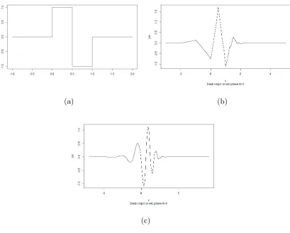
One of the major weaknesses of the Discrete Wavelet Transform is that it is not translation-invariant, this means that if we take the DWT of an input vector and then shift this input vector by some amount and again perform the transform then we will obtain different results. This is not an attractive quality for a wavelet transform to possess since it means that analysis using this transform will be affected by the choice of origin. An example of this can be seen in Figure 2.1.3; shifting the original data by one to the left results in completely different wavelet coefficients. ThewavethreshR package (Nason, 2016) was used to apply the wavelet transform and generate the plots of the wavelet decomposition coefficients. The Non-decimated Wavelet Transform (NDWT) was developed as a solution to this problem and will be outlined in the next section.

2.1.5

Non-decimated Wavelet Transform (NDWT)

(a) (b)

(c) (d)

Figure 2.1.3: Example of the lack of translation-invariance of the DWT; (a) shows the original data whilst (b) shows the data rotated by a unit shift. Figures (c) and (d) depict the Haar DWT for the original and shifted data respectively.

is carried out which means that the number of smooth and detail coefficients does not change at each level of the process.

At each step of the NDWT we have to pad the high and low pass filters with zeroes. Let H = {hk}k∈Z be the initial low-pass filter and let G = {gk}k∈Z be the

high-pass filter. Following the notation of Nason and Silverman (1995), we define the filtersH[r] _{and G}[r] _{which consist of the elements}

h[r]₂r_j =hj,

h[r]_k = 0,

g₂[r]r_j =gj,

g_k[r]= 0, if k is not a multiple of 2r.

(2.1.27)

between every adjacent element of the filterH[r−1] _{which is used at the previous step} of the algorithm. As in Section 2.1.4, let cJ _={c

J,k}k be the initial data vector. The smooth and detail coefficients at scale j−1 are given by

c(j−1) =H[J−j]c(j), (2.1.28)

d(j−1) =G[J−j]c(j), (2.1.29) wherec(j) is the vector of smooth coefficients at scalej andd(j) is the vector of detail coefficients. The operatorH[r]_{can be thought of as the convolution operator with the} filter h(r)_.

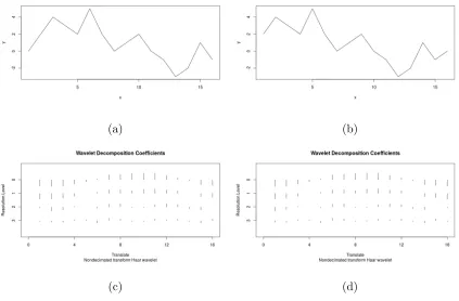
One of the major strengths of the NDWT, in comparison to the DWT, is that it includes extra information from the data at coarser scales, since no decimation step is carried out. Any information contained in the odd-indexed elements is included in the transform and not discarded, therefore each level of the transform will have coefficients for all locations k ∈ {0, . . . , T −1}. In addition to this, the NDWT is translation-invariant and so is not affected by the choice of origin of the input data.

consequence of this, the NDWT does not have a unique inverse and so the algorithm is not easily invertible. A number of approaches have been developed for inverting the NDWT including the Average Basis method of Coifman and Donoho (1995) or using the algorithm of Coifman and Wickerhauser (1992) to select a best basis and reconstructing the signal from this.

(a) (b)

(c) (d)

Figure 2.1.4: Example of the translation-invariance of the NDWT; (a) shows the original data whilst (b) shows the data rotated by a unit shift. Figures (c) and (d) depict the Haar NDWT for the original and shifted data respectively.

relaxing the restriction that the input data must be dyadic length, see Percival and Walden (2006) for a complete description. Another example is the wavelet packet transform of Coifman and Wickerhauser (1992). This is a generalization of the dis-crete transforms discussed above in which the low and high-pass filters are applied to both the smooth and detail coefficients and these are then carried forward to the next level of the transform. As with the NDWT, if all of the wavelet packets are included in the decomposition then it can be seen that this is an overcomplete trans-form. However Coifman and Wickerhauser (1992) proposed the best basis algorithm to select which packets are best for representing the series and forming an orthogo-nal transform. Fiorthogo-nally, the lifting scheme, introduced in Sweldens (1996, 1998), can be used to produce a multi-scale decomposition of signals observed on an irregularly spaced grid or containing missing data in a computationally efficient manner.

2.2

Time Series Analysis

We now turn our attention to some key time series analysis concepts relevant for this thesis. A time series is a collection of observations of a process made sequentially through time. These measurements can either be taken continuously through time or at discrete, successive time points. Within this thesis, we focus on discrete time series

{xt}t∈N. A comprehensive overview of time series analysis concepts can be found

One of the most widely covered topics within time series analysis is that of sta-tionarity, in particular stationary time series modelling. Informally, one can consider a stationary time series to be one whose statistical properties do not change over time. More specifically, following Shumway and Stoffer (2000), a time series is said to be strictly stationary if the probabilistic behaviour of every subset of values

{xt1, xt2, . . . , xtk}

is the same as that of the time shifted subset

{xt1+h, xt2+h, . . . , xtk+h}.

This can be expressed as,

P(xt1 ≤c1, . . . , xtk ≤ck) =P(xt1+h ≤c1, . . . , xtk+h ≤ck)

for allk = 1,2, . . . , all time pointst1, t2, . . . , tk, all time shifts h= 0,±1,±2, . . . ,and all constants c1, c2, . . . , ck.

In practice, these strict assumptions of stationarity can often be too restrictive and so we consider an alternative; that of second order stationarity. A process is said to be second order stationary if it has constant mean and the covariance between observations depends only on the lag between them and not on time, in other words

E[xt] =µ, and γt(τ) = cov(xt, xt+τ) = κτ.

modelling stationary time series and efficiently capturing their dependence structure is an important one, we will now review some popular time series models in Section 2.2.1.

2.2.1

Stationary time series modelling

There are many existing stationary time series models within the literature that incor-porate some degree of changing dependence; some focus on modelling the behaviour of the series in the time domain whereas others concentrate on the frequency domain.

Stationary processes in time domain

Popular approaches to modelling univariate stationary processes in the time domain include the moving average processes and the autoregressive processes, introduced in Yule (1927). A moving average process of order q, denoted MA(q), is a linear combination of the current innovation term and the q most recent innovations. The tth _{observation of the process takes the form}

Xt=t+θ1t−1+. . .+θqt−q (2.2.1) where t are iid white noise processes with variance σ2 for all t∈ N and {θt}t∈{1,...,q}

is the set of MA coefficients.

In a similar way, an autoregressive process of order p is a linear combination of the current innovation term and the pmost recent observations. The tth _observation of the process takes the form

where againtare iid white noise processes with varianceσ2 and theφi are the model parameters withφp 6= 0 for an order p process.

Whittle (1951) combined the MA and AR processes to form the autoregressive moving average (ARMA) processes. Thetth observation of an ARMA(p, q) process is given by

Xt=φ1Xt−1+φ2Xt−2+. . .+φpXt−p+t+θ1t−1+. . .+θqt−q (2.2.3) where p and q are the AR and MA orders respectively and is white noise with varianceσ2_.

For a stationary time series, the autocorrelation and partial autocorrelation func-tions can be used to estimate the values ofpandqto be used in the ARMA model. The Box-Jenkins methodology is commonly used to fit the stationary time series model and estimate the AR and MA model parameters, further details on this method can be found in Chatfield (2004) and Box et al. (2015).

All of the models described above are univariate and could be applied to individual components of a multivariate time series however this would not account for any dependencies between the components. For this reason, multivariate extensions of the above models have been proposed in the literature. By way of introduction, we briefly outline the vector autoregressive moving average processes. Interested readers can find further details in Tiao and Tsay (1989) and L¨utkepohl (2007).

inno-vations. Thetth observation of an m-dimensional VARMA(p, q) process Xt takes the form

Xt=A1Xt−1+. . .+ApXt−p+Zt+M1Zt−1+. . .+MqZt−q (2.2.4) where {Al}l∈1,...,p and {Ml}l∈1,...,q are (m×m) matrices of AR and MA coefficients respectively which capture the temporal dependence of the multivariate time series. In this case,Zt is a (m×1) innovation vector with mean 0 and covariance matrix Σ.

Stationary processes in frequency domain

Within the frequency domain, the Fourier basis has been used to construct represen-tations of stationary univariate processes, see Priestley (1981) for a comprehensive description.

A zero-mean stationary stochastic process Xt can be represented in the following way within the Fourier setting

Xt =

Z π

−π

A(ω)exp(iωt)dξ(ω) for t∈_Z and ω∈[−π, π]. (2.2.5)

Here, A(ω) is the amplitude of the process, exp(iωt) is the oscillation and dξ(ω) is an orthonormal increments process. The spectrum of a process provides information on the power of the process at a given frequency. More precisely, for a time series of lengthT, the spectrum at frequency ω of a stationary process X is given by

fX(ω) = T

∞

X

τ=−∞

γ(τ) exp(−iωτ T) (2.2.6)

terms of the spectrum in the following way

γ(τ) = 1 T

Z

fX(ω) exp(iωτ T)dω. (2.2.7)

2.2.2

Nonstationary time series modelling

In practice, many of the time series observed from industrial and other applications are nonstationary. I.e. their second order structure evolves over time. When the stationarity assumptions no longer hold, the previously described models should not be applied in their standard forms because poor estimates of the model parameters will be produced and the nonstationarity will not be accurately captured. Consequently, further thought is required to model the changing second order behaviour. One way to achieve this would be to adapt the ARMA framework to allow the model coefficients to change over time, see Subba Rao (1970) and Grenier (1983) for details on how to estimate these coefficients. In this section, we review some more recent approaches to modelling nonstationary time series using a variety of basis functions, including the Locally Stationary Fourier processes and the Smooth Localized Exponential (SLEX) model.

Locally Stationary Fourier processes

{Xt,T}Tt=0−1 can be represented as follows Xt,T =

Z π

−π

A0_t,T(ω)exp(iωt)dξ(ω) (2.2.8)

where{exp(iωt)}ωis a set of harmonics andA0t,T(ω) is the transfer function. A number of smoothness conditions are imposed onA0_t,T(ω) to ensure that the amplitude is not too irregular over time. Further details on these conditions can be found in Definition 2.1 of Dahlhaus (1997). The representation in equation (2.2.8) assumes that the series is locally stationary, that is, if we observed the series at sufficiently small intervals then it would appear stationary.

Within the LSF framework, Dahlhaus (1997) introduced the concept of rescaled time. In other words, rather than observing a time series and the amplitude over a grid t ∈ {1, . . . , T}, instead observe them on the interval u = t/T ∈ [0,1]. In this setting, increasing the number of observations T corresponds to observing the series on a finer grid. This mathematical construct is important, as it enables us to establish theoretical guarantees about the behaviour of LSF estimates.

Dahlhaus (2000) presents the multivariate generalization of the univariate local stationarity described above. It is shown that there exists a locally stationary repre-sentation analogous to that in equation (2.2.8) for Gaussian multivariate series and time-varying MA(∞) processes. For a d-dimensional series, the univariate transfer function is replaced with a (d×d) transfer function matrix A0 where smoothness con-ditions are imposed on each entry A0

Smooth Localized Exponential (SLEX) model

The LSF framework is by no means the only representation of a locally stationary time series. For example, Ombao et al. (2002) build on the Locally Stationary Fourier model of Dahlhaus (1997) to provide an alternative locally stationary representation of a nonstationary process. Within the time series literature, windowed or tapered Fourier exponentials have traditionally been used to model and analyse nonstationary processes (Daubechies, 1992). These functions take the form

φF(u) = Ψ(u)exp(i2πωu) (2.2.9)

where Ψ is a taper with compact support andω ∈(−1 2,

1

2]. The main drawback associ-ated with the windowed Fourier exponentials is that, whilst they are localized in time, they are not necessarily orthogonal (Wickerhauser, 1994). Ombao et al. (2002) replace the set of Fourier complex exponential basis functions within the Locally Stationary Fourier representation of equation (2.2.8) by the Smooth Localized Complex Expo-nential (SLEX) basis functions in order to overcome this problem. Their approach preserves the orthogonality of the basis functions through the use of a projection op-erator, rather than applying a single taper. This projection operator has the same effect as applying two smooth and compactly supported windows to the Fourier basis functions.

has elements {φS,ωk(t)} where

φS,ωk(t) = φωk

t−α0

|S|

!

= Ψ+

t−α0

|S|

!

exp(i2πωk(t−α0)) + Ψ−

t−α0

|S|

!

exp(−i2πωk(t−α0))

(2.2.10)

where ωk = k

|S| and k = − |S|

2 + 1, . . . ,

|S|

2 . A complete description of the locally stationary SLEX model can be found in Ombao et al. (2002), including a description of how to select the best SLEX basis for the particular time series.

A multivariate extension of the SLEX model was introduced by Ombao et al. (2005), in which the scalar transfer functions used within the locally stationary uni-variate representation are again replaced by (d×d) transfer function matrices defined on particular blocks. In addition, the cost function used to determine the best SLEX model for the time series is modified to take into account auto and cross-correlation information from all channels.

2.3

Wavelets in Time series

the other hand, whilst the SLEX model is computationally efficient, the requirement that the stationary blocks that segment the time series must be of dyadic length can be restrictive. In this section, we discuss an alternative model that is built on non-decimated wavelets, called the Locally Stationary Wavelet model. We then discuss the multivariate generalization, the Multivariate Locally Stationary Wavelet model, which is used within the time series classification and imputation methods outlined in Chapter 3 and 4 respectively.

2.3.1

Locally Stationary Wavelet model

The Locally Stationary Wavelet (LSW) processes, introduced by Nason et al. (2000), can be used to model a nonstationary time series with changing second order structure. The model has as its building blocks the discrete non-decimated wavelets which are compactly supported and localized in time and scale. A LSW process{Xt,T}_{t=0,...,T−1}, T = 2J _{≥1 is formally defined as follows}

Xt,T =

∞

X

j=1

X

k

Wj(k/T)ψjk(t)ξjk. (2.3.1)

Here,{ψjk(t)}_jk is a collection of discrete non-decimated wavelets,ξjk is a random or-thonormal increments sequence and{Wj(k/T)}is a set of amplitudes. Consequently, the time series is modelled as the sum of a collection of non-decimated wavelets

{ψjk(t)}_jk (oscillations) which have random amplitudes{Wj(k/T)ξjk}.

(2000), these assumptions are

1. E(ξjk) = 0 for all j and k.

2. cov(ξjk, ξlm) = δjlδkm, whereδjk is the Kronecker delta.

3. There exists a Lipschitz continuous function Wj(z) for each j ≥ 1, z ∈ (0,1) which satisfies the following properties:

(a) X j

|Wj(z)|2<∞ uniformly in z ∈(0,1),

(b) The Lipschitz constants Lj are uniformly bounded in j and

X

j

2jLj <∞.

(c) There exists a sequence of constantsCj such that for each T

sup k

wj,k;T −Wj

k T

≤ Cj

T

where for each j = 1, . . . , J(T) = log₂(T) the supremum is over k = 0,1, . . . , T −1, and where{Cj} fulfils

X

j

Cj <∞.

The first assumption ensures that the LSW process has mean zero and the second ensures that the orthonormal increments sequence is uncorrelated. The third as-sumption controls how the amplitudes change over time, with the amplitudes wj,k:T behaving similarly to some transfer functionWj(z), which in turn is controlled so that it does not oscillate too rapidly.

evolutionary wavelet spectrum (EWS). The EWS provides information about the power of the process at scalej and location z wherez = _Tk is the rescaled time. This has the form

Sj(z) =|Wj(z)| 2

(2.3.2)

for scalejand rescaled timez. As in the Fourier setting, Nason et al. (2000) show that the autocovariance of function of a series can be written in terms of the EWS, similarly to equation (2.2.7). The local autocovariance (LACV) function gives information on the covariance of an LSW process around a location z = k/T ∈ (0,1). The LACV can be written as

c(z, τ) = cov(X[zT], X[zT]−τ) =

∞

X

j=1

Sj(z)Ψj(τ) (2.3.3)

where the autocorrelation wavelets Ψj(τ) are given by

Ψj(τ) =

X

k

ψjk(0)ψjk(τ). (2.3.4)

Estimation of the EWS

The first step towards estimating the EWS is to calculate the empirical wavelet coef-ficients of Xt,T, which are defined to be

dj,k = T−1

X

t=0

Xt,Tψjk(t). (2.3.5)

The raw wavelet periodogram of a LSW process Xt,T is then given by

Nason et al. (2000) show that the (asymptotic) mean and variance of the raw wavelet periodogram have the form

E[Ij,k] =

X

l

Aj,lSl(z) +O(T−1), (2.3.7) var[Ij,k] = 2n X

l

Aj,lSl(z)

o2

+O

2j T

. (2.3.8)

Note thatAj,l refers to the (j, l) entry of the inner product matrix A of the autocor-relation wavelets, defined by

Aj` =hΨj,Ψ`i=

X

τ

Ψj(τ)Ψ`(τ) (2.3.9)

where Ψ are the autocorrelation wavelets as defined in equation (2.3.4).

It can be seen from equation (2.3.7) and (2.3.8) that the raw wavelet periodogram is an asymptotically biased and inconsistent estimator of the EWS. Nason et al. (2000) propose smoothing the raw wavelet periodogram before correcting by A−1 to obtain a consistent and unbiased estimator. Smoothing the raw wavelet periodogram can be done in a number of ways, Nason et al. (2000) use the translation-invariant denoising of Coifman and Donoho (1995) but alternative methods can be found in Fryzlewicz and Nason (2006) and Van Bellegem and Von Sachs (2008).

(a) An example of an EWS (b) One realisation of this process

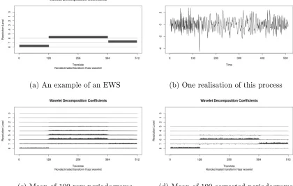
(c) Mean of 100 raw periodograms (d) Mean of 100 corrected periodograms

Figure 2.3.1: Example showing the effect of correcting the raw wavelet periodograms.

the mean of the 100 raw wavelet periodograms, from this we can see the bias in the raw periodogram as power has leaked into surrounding scales. Correcting the raw wavelet periodogram removes most of this bias, Figure 2.3.1(d) shows the mean of the 100 corrected wavelet periodograms. We can see that most of the power leakage has disappeared and the corrected periodogram is much closer to the true EWS.

2.3.2

Multivariate Locally Stationary Wavelet framework

components of the series. This framework allows each individual component of the time series to exhibit nonstationary behaviour, which is captured by the model in addition to the cross-dependence structure between components. A similar model is developed in Cho and Fryzlewicz (2015) however this is restricted to the context of changepoint detection of piecewise stationary signals.

Suppose that we have aP-variate input vector of the form Xt,T ={X (1) t,T, X

(2) t,T, . . . ,

X_t,T(P)}>_{. Each element X}(i)

t,T (for i = 1,2, . . . , P) is a univariate component of the signal, known as a channel. The transfer function,Wj(k/T), from the univariate case is replaced by a P ×P transfer matrix of functions, denoted Vj(k/T). The random orthonormal increments sequence, ξjk, is replaced by a set of random vectors of the form{zj,k}=

n

[z_j,k(1), z(2)_j,k, . . . , z_j,k(P)]>o.

Following Park et al. (2014), a P-variate locally stationary wavelet process

{Xt,T}t=0,1,...,T−1, T = 2J ≥1 has the following representation

Xt,T =

∞

X

j=1

X

k

Vj(k/T)ψj,t−kzj,k, (2.3.10) whereVj(k/T) is the transfer function matrix and{ψj,t−k}j,k is a set of discrete non-decimated wavelets. There are a number of conditions required of the quantities in equation (2.3.10) analogous to those for the univariate LSW case. Specifically, the random vectors, zj,k, are uncorrelated, have mean vector 0 and variance-covariance matrix equal to the P ×P identity matrix. The lower-triangular transfer function matrix must be made up of Lipschitz continuous functions with Lipschitz constants Lj that satisfy

X

j

The time-dependent transfer function matrix, Vj(k/T), encapsulates both the be-haviour of the individual channels and the cross-channel dependence over time. The spectral structure of the multivariate time series is important as this provides informa-tion on the time-scale decomposiinforma-tion of power within the series; the transfer funcinforma-tion matrix is key to determining this structure. In particular, given a multivariate LSW signal,Xt,T, with transfer function matrix,Vj(k/T), the local wavelet spectral (LWS) matrix is given by

Sj(z) = Vj(z)Vj(z)> (2.3.11) where j is the scale and z = _Tk is the rescaled time. As in the univariate setting, the local auto and cross-covariance of a multivariate LSW series can be expressed in terms of the LWS matrix. Following Park et al. (2014), let c(p,p)_{(z, τ) denote the} local autocovariance of channel p at lag τ and let c(p,q)_{(z, τ) denote the local} cross-covariance between channels p and q. The local auto and cross-covariance functions are then defined to be

c(p,p)(z, τ) =

∞

X

j=1

S_j(p,p)(z)Ψj(τ), (2.3.12)

c(p,q)(z, τ) =

∞

X

j=1

S_j(p,q)(z)Ψj(τ). (2.3.13)

Here Ψ are the discrete autocorrelation wavelets.

the cross-spectra between channels. Using the notation of Park et al. (2014), we de-note the spectra of the individual channel p by S(p,p)_j and the cross-spectra between channelsp and q as S(p,q)_j .

A key strength of the mvLSW framework is that it provides a way to model time-varying dependence structure between channels. The concept of wavelet coherence was originally introduced in the bivariate setting in Sanderson et al. (2010), Park et al. (2014) extend this to the multivariate setting using the mvLSW framework. The wavelet coherence is defined to be the linear relationship between two channels, including any indirect links between them that depend on other channels of the signal. The wavelet coherence matrix,ρj(z), at scale,j, and rescaled time, z, can be defined in terms of the local wavelet spectral matrix and has the form

ρ_j(z) =Dj(z)Sj(z)Dj(z), (2.3.14)

where,Sj(z), is the local wavelet spectral matrix andDj(z) is a diagonal matrix with elementsS(p,p)_j (z)(−1/2)_{. Individual elements of the coherence matrix have the form}

ρ(p,q)_j (z) = S (p,q) j (z)

q

S_j(p,p)(z)S_j(q,q)(z)

, (2.3.15)

whereρ(p,q)_j (z) is the coherence between channel p and q for scale j, at rescaled time z ∈ (0,1). The coherence takes a value between −1 and 1 where a value of ±1 shows a strong positive/negative linear relationship between channels at that scale and time. On the other hand, a value close to 0 indicates that there is very little linear dependence between channels.

this, Park et al. (2014) introduce the concept of wavelet partial coherence which is a measure of the coherence between two channels after removing the effects of all other channels. The wavelet partial coherence matrix at scale, j, and rescaled time, z, is defined to be

Γj(z) = −Hj(z)Gj(z)Hj(z) (2.3.16)

whereGj(z) =Sj(z)−1 and Hj(z) is a diagonal matrix with entries G (p,p) j (z)

−1/2_.

Estimation of the LWS

We can estimate the spectral properties of a multivariate signal by first calculating the empirical wavelet coefficients for each channel of the signal, and then using this to obtain the raw wavelet periodogram. More formally, the empirical wavelet coefficient vector,dj,k =

n

d(1)_j,k, d(2)_j,k, . . . , d(P_j,k)

o>

, is given by

dj,k = T−1

X

t=0

Xtψj,k(t). (2.3.17)

This can then be used to obtain the raw wavelet periodogram matrix,Ij,k, which has the following form

LWS. In particular, they show that

E[Ij,k] = J

X

l=1

Aj,lSl(k/T) +O(T−1), (2.3.19) var(I_j,k(p,q)) =

J

X

l=1 Aj,lS

(p,p) l (k/T)

J

X

l=1 Aj,lS

(q,q) l (k/T)

+ J

X

l=1

Aj,lS_l(p,q)(k/T)

!2

+O(22j/T).

(2.3.20)

To account for this, the raw wavelet periodogram must be smoothed and cor-rected in some way. Park et al. (2014) propose smoothing the periodogram using a rectangular kernel smoother with window length 2M + 1 to obtain the estimator

˜_{Ij,k =} 1 2M + 1

M

X

m=−M

Ij,k+m. (2.3.21)

The bias of the smoothed wavelet periodogram ˜I can be corrected using the inverse of the inner product matrix in order to give a consistent and unbiased estimate of the LWS matrix ˆS with entries given by

b

Sj,k = J

X

l=1

A−_jl1I˜l,k. (2.3.22) The wavelet coherence matrix can then easily be estimated by substituting ˆS into equation (2.3.14).

2.4

Classification of nonstationary time series

briefly review some approaches to do this both in the univariate and multivariate contexts.

2.4.1

Static classification

We first consider static classification approaches in which an entire nonstationary signal is assigned to one particular class. In this situation, the class membership of the test signal is not permitted to vary over time. We will summarise a number of classification methods which are based on the nonstationary models described in Section 2.2.2 including the SLEX-based method of Huang et al. (2004) and the LSW-based approaches of Fryzlewicz and Ombao (2009) and Krzemieniewska et al. (2014). The classification method introduced in Huang et al. (2004) uses the SLEX model to classify an unseen test signal using information from a set of (univariate) training signals of known class membership. The first step of the algorithm involves determin-ing the best basis representation of each traindetermin-ing signal from the SLEX library before estimating the SLEX periodograms based on these chosen representations. These pe-riodograms are then averaged over the signals known to belong to each class to obtain estimates of the spectral information. An unseen time series is then assigned to a class, Πc, if the Kullback-Liebler divergence between its estimated spectrum and the spectrum of Πc is smaller than that between the estimated spectrum and the spectra of any other class.

Ombao (2009) proposed an LSW-based alternative that overcomes this restriction. Again, the first step of this approach involves calculating the empirical wavelet spec-trum,Lj,k =P_i(A−1)i,jIi,k,whereIi,k is defined as in equation (2.3.6). The empirical wavelet spectra are then averaged over the training signals known to belong to classc in order to estimate the evolutionary wavelet spectrum, denoted ˆS_j(c)(z). The discrim-inating set,M, is then determined by choosing a specified proportion of the timescale indices (j, k) that maximise the divergence index

∆(j, k) = G

X

g=1

"

ˆ

S_j(g)(k/T)− 1

G G

X

h=1 ˆ

S_j(h)(k/T)

#2

. (2.4.1)

In order to classify a time series, Fryzlewicz and Ombao (2009) first estimate its empirical wavelet spectrum, Lj,k, and then calculate the following squared distances for each classg

Dg =

X

(j,k)∈M

(Lj,k −Sˆ (g)

j (k/T)) 2

. (2.4.2)

The time series is then assigned to the class g that minimises the above distance measure.

Whilst this method works well when each of the class generators produce spectra with equal variability across realizations, when this is not the case choosing the most divergent coefficients may not be the best approach for classification. Krzemieniewska et al. (2014) proposed an extension to the work of Fryzlewicz and Ombao (2009) that accounts for within-class variation between signals. As in Fryzlewicz and Ombao (2009), the empirical wavelet spectra for each class is estimated by averaging the periodograms for the time series replications known to belong to that class. Krzemie-niewska et al. (2014) then estimate the variability at different scales and locationsσ2

in the following way

σ2_j,k = _Pc1 g=1Ng

c X g=1 Ng X n=1

(Lg,n_j,k −Sˆ_j(g)(k/T))2

. (2.4.3)

The subset of discriminating coefficients, M, is chosen by selecting pairs (j, k) that maximise the alternative divergence index

˜

∆(j, k) = ∆(j, k)/σ_j,k2 . (2.4.4)

Here, ∆(j, k) is defined in equation (2.4.1). The modified distance for an observed signal is given by

˜ Dg =

X

(j,k)∈M

(Lj,k −Sˆ (g)

j (k/T)) 2 σ2

j,k

. (2.4.5)

The signal is then assigned to the classg for which ˜Dg is smallest.

2.4.2

Dynamic classification

(2018) apply a Fisher z transform to the coherence estimates in order to ensure that they can be approximated by a Gaussian distribution. For a classc, the transformed coherence ξ_j(c) is given by

ξ_j(c) = tanh−1ρ(c)_j . (2.4.6) The mean and variance of the transformed coherence for classccan be estimated using the transformed coherence for the training signals that are known to belong to that particular class. In a similar way to the static classification method of Krzemieniewska et al. (2014), these mean and variance estimates are used to determine the subset of coefficients that show the largest difference between the classes in terms of the transformed coherence. In the multivariate setting, the subsetMconsists of the scale and channel indices, (j, p, q), for p < q that maximise the discrepancy measure ∆(p,q)_j which is given by

∆(p,q)_j = Nc X c=1 Nc X g=c+1

ξ_j(p,q)(c)−ξ_j(p,q)(g)

q

var(ξ(p,q)(c)_j ) + var(ξ_j(p,q)(g))

. (2.4.7)

As the class membership of the observed signal is allowed to change over time, this approach estimates the probability that the signal belongs to a particular class at a given time. Park et al. (2018) first estimate the transformed coherence for the signal Xt, denoted ˆξj,k;X. Bayes’ theorem is then used to estimate the probability that the signal belongs to classc at a particular time given prior information in the following way

PrhC(k) =c|ξˆj,k;X

i

∝Pr [C(k) = c]L( ˆξj,k;X|ξj(k/T) =ξ (c)

j ∀ j) (2.4.8)

at rescaled time k. This is typically assigned the probability of _N1

c provided that no

Dynamic detection of anomalous

regions within distributed acoustic

sensing data streams using locally

stationary wavelet time series

3.1

Introduction

The ability to accurately analyse geoscience data at, or close to, real time is becoming increasingly important. For example, within the oil and gas sector this need can arise as a consequence of (i) the sheer volume of data now being collected and (ii) operational considerations. It is this setting that we consider in this article, seeking to enable the rapid identification of certain anomalous features within Distributed Acoustic Sensing data obtained from an oil producing facility. Specifically, we seek to

build on recent work within the nonstationary time series community to develop an approach that permits the online monitoring of these complex signals.

The technology used to generate the data considered in this article, Distributed Acoustic Sensing (DAS), involves the use of a fibre-optic cable as a sensor in which the entire length of the fibre is used to measure acoustic or thermal disturbances. DAS originates from the defence industry where it is commonly used in security and border monitoring (Owen et al., 2012). Recently, the technology has been applied within the oil and gas industry, for example in pipeline monitoring and management (Williams, 2012; Mateeva et al., 2014). The use of DAS to monitor production volumes and composition within a well requires the installation of a fibre-optic cable along the length of the well combined with an interrogator unit on the surface (Paleja et al., 2015). This unit sends light pulses down the cable and processes the back-scattered light. The installation of such technology has become popular as it is can be a cost effective way to obtain continuous, real-time and high-resolution information.

physical. Instead stripes can occur for a number of reasons, including a disturbance of the fibre-optic cable near the unit, or problems with the electronics due to the high sampling rate.

Visually, stripes can manifest themselves in a variety ways. Some are visually obvious within the DAS data, such as the stripe that occurs at around 4000ms in Figure 3.1.1(a). Other occurrences can be more subtle, and therefore more challenging to detect. For example, the stripe could be a change in the second-order structure. Critically such features can make it difficult to carry out further analysis of the data, such as flow rate analysis. For this reason, there is significant interest in being able to detect regions of striping as soon as they occur, so that they can be removed whilst keeping as much of the original signal intact as possible. It is this challenge of dynamically detecting striping regions that motivates the work presented in this article.

(a)

(b)

(a)

(b)

a recent overview of classification in the time series context, see for example Fu (2011). Dependent on the application being considered, one might adopt various modelling choices. For example, some classifiers have distinct advantages, such as simplicity of implementation, speed or suitability for massive online applications. However many, such as GMM or SVM-based approaches, do not explicitly allow temporal dependence or are limited to a narrow class of series structure (HMMs), which is seen as crucial to classification of time series in the majority of realistic settings (see e.g. Bifet et al. (2013)). Complex hidden dependence structure is typical of the DAS data studied in this article (see Figure 3.1.2).

Our approach to the dynamic stripe identification problem builds on recent work within the time series literature. Wavelet approaches to modelling time series have become very popular in recent years, principally because of their ability to provide time-localised measures of the spectral content inherent within many contemporary data (e.g. Killick et al. (2013); Nam et al. (2015); Chau and von Sachs (2016); Nason et al. (2017)). Thislocally stationary modelling paradigm is flexible enough to repre-sent a wide range of nonstationary behaviour and has also been extended to enable the modelling and estimation of multivariate nonstationary time series structures (e.g. Sanderson et al. (2010) and Park et al. (2014)). Typically these settings assume that the data have already been collected, and are available for offline analyses.

dependencies both within and between channels of the series, including those which exhibit visually subtle changes in behaviour over time. Reusing data calculations al-lows us to also produce a computationally efficient nondecimated wavelet transform in the online setting.

This work is organised as follows. In Section 3.2, we describe the proposed online classification method. Section 3.3 contains a simulation study evaluating the perfor-mance of the proposed classifier using synthetic data, further justifying the use of time-varying coherence as a feature for classification. A case study using an acoustic sensing dataset is then described in Section 3.4, where we discuss the utility of the proposed classifier as a stripe detection method. Finally, Section 3.5 includes some concluding remarks.

3.2

Online dynamic classification of multivariate

series

In order to adapt the existing dynamic classification method outlined in Section 2.4.2 to an online setting, we make use of a moving window approach. The use of such a window encapsulates the constraint in many data streaming applications that there is only limited data storage and memory with which to perform analysis.