Decoupling Encoder and Decoder Networks for
Abstractive Document Summarization
Ying Xu1, Jey Han Lau2,3, Timothy Baldwin3andTrevor Cohn3 1Monash University
2IBM Research
3The University of Melbourne
[email protected], [email protected] [email protected], [email protected]
Abstract
Abstractive document summarization seeks to automatically generate a sum-mary for a document, based on some abstract “understanding” of the original document. State-of-the-art techniques tra-ditionally use attentive encoder–decoder architectures. However, due to the large number of parameters in these models, they require large training datasets and long training times. In this paper, we propose decoupling the encoder and decoder networks, and training them separately. We encode documents using an unsupervised document encoder, and then feed the document vector to a recurrent neural network decoder. With this decoupled architecture, we decrease the number of parameters in the decoder substantially, and shorten its training time. Experiments show that the decoupled model achieves comparable performance with state-of-the-art models for in-domain documents, but less well for out-of-domain documents.
1 Introduction
Abstractive document summarization is a chal-lenging natural language understanding task. Ab-stractive methods first encode the original docu-ment into a high-level representation, and then de-code it into the target summary.
Rush et al. (2015) proposed the task of head-line generation as the first step towards abstrac-tive summarization. Instead of using the full docu-ment, the authors experimented with using the first sentence as input, with the aim of generating a co-herent headline given the sentence.
The current state-of-art system for the task is based on an attentive encoder and a recurrent de-coder (Chopra et al., 2016), which is an extension of the methodology of Rush et al. (2015). The encoder and decoder are trained jointly, and the decoder attends to different parts of the document during generation. It has a large number of param-eters, and thus requires large-scale training data and long training times.
In this paper, we propose decoupling the en-coder and deen-coder. We encode documents using
doc2vec (Le and Mikolov, 2014), as it has been
demonstrated to be a competitive unsupervised document encoder (Lau and Baldwin, 2016). We incorporate doc2vec vectors of input documents
to the decoder as an additional signal, to gener-ate sentences that are not only coherent but are also related to the original documents. Compared to the standard joint encoder–decoder design, the decoupled architecture has less parameters for the decoder, and thus requires less training data and trains faster.1 The downside of the decoupled ar-chitecture is that thedoc2vecsignal is not updated
in the decoder, and its document representation could be sub-optimal for the decoder to generate good summaries. Our experiments reveal that the decoupled architecture works well in-domain, but less well out-of-domain, as a consequence of the fixed capacity of the document encoding as well as having no explicit copy mechanism.
2 Attentive Recurrent Neural Network: A Joint Encoder–decoder Architecture
The attentive recurrent neural network is com-posed of an attentive encoder and a recurrent de-coder (Chopra et al., 2016), where the ende-coder is
1The training time is decreased from 4 days (with full GI
-GAWORD) for the coupled model (Rush et al., 2015) to 2 days (with 75% GIGAWORD) in our model with comparable in-domain performance.
!(#$|#&, … , #$)&, *; ,)
.$ ℎ$
01.2345 #$)&
Decoder Encoder
* !(#$)&|#&, … , #$)6, *; ,)
.$)& ℎ$)&
01.2345 #$)6
*
(a) Joint encoder–decoder architecture
!(#$|#&, … , #$)&, *; ,)
ℎ$
#$)&
Decoder Encoder
!(#$)&|#&, … , #$)6, *; ,)
ℎ$)&
01.2345 #$)6
* To hidden unitTo softmax layer
doc2vec
[image:2.595.105.497.74.199.2](b) Decoupled encoder–decoder architecture
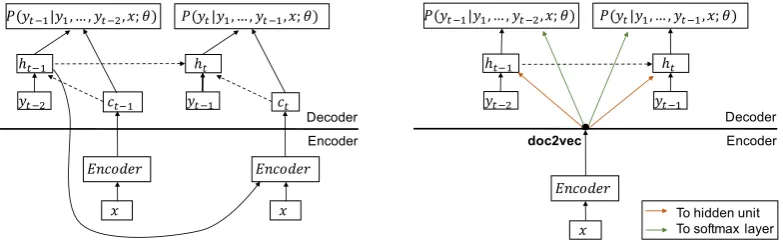
Figure 1: Encoder–decoder architectures
a fixed-window feed-forward network and the de-coder is a recurrent neural network (RNN: Elman (1998), Mikolov et al. (2010)) language model and parameters from both networks are trained to-gether. Let x denote the document, y the sum-mary,θthe set of parameters to be learnt, andy=
y1, y2, ..., yN a word sequence of lengthN. When decoding, y is computed as argmaxP(y|x;θ), where the conditional probability P(y|x;θ) can be calculated from each wordyt in the sequence, i.e.P(y|x;θ) =QNt=1P(yt|{y1, ..., yt−1},x;θ).
For the recurrent decoder, the condi-tional probability of each word is given as
P(yt|{y1, ..., yi−1},x;θ) = gθ(ht,ct), where ht represents the hidden state of RNN, i.e. ht = gθ(yt−1,ht−1,ct), andctthe output of the encoder at timet.
For the attentive encoder,xis computed by at-tending to some of the source words using the pre-vious hidden stateht−1.2 Figure 1a demonstrates
the dependencies between the next generated word
ytand documentx, given the parametersθ. The decoupled architecture ensures that the in-formation from documentxis adapted to the cur-rent context of the generated summary.
3 Decoupled Encoder–decoder Architecture for Document Summarization
A decoupled encoder–decoder architecture has a clear boundary between the encoder and decoder: it can be seen as a pipeline model where the output of the encoder is fed as an input to the decoder, so
2The unnormalised attention weights are computed by
combininght−1 with the convolutional embedding of each source word via dot product.
the encoder and decoder modules can be trained separately. Figure 1b illustrates how the encoder and decoder are decoupled from each other. Here, we usedoc2vecthe document encoder and a
long-short term memory network (LSTM: Hochreiter and Schmidhuber (1997)) as the decoder.
doc2vecis an extension ofword2vec(Mikolov
et al., 2013), a popular deep learning method for learning word embeddings. In word2vec (based
on theskipgramvariant) the embedding of a
tar-get word is learnt by optimising it to predict its position-indexed neighbouring words. doc2vec
(based on thedbowvariant) is based on the same
idea, except that the target word is now the docu-ment itself, and the docudocu-ment vector is optimised to predict the document words. Note that thedbow
implementation does not take into account the or-der of the words (hence its name “distributed bag of words”). Once the model is trained, embed-dings of new/unseen documents can be inferred from the pre-trained model efficiently. As an en-coder, doc2vec is completely unsupervised, and
uses no labelled information or signal from the de-coder.
The decoder is an RNN language model (Mikolov et al., 2010), implemented as an LSTM (Hochreiter and Schmidhuber, 1997). Formally:
it=Wixt+Uiht−1+bi ft=Wfxt+Ufht−1+bf ot=Woxt+Uoht−1+bo
jt=Wjxt+Ujht−1+bj
ct=ct−1∗σ(ft) + tanh(jt)∗σ(it)
ht= tanh(ct)∗σ(ot)
(1)
Combination Equation
add-input i0t =it+d
add-hidden h0
t =ht+d
stack-input i0t = [it;d] stack-hidden h0t = [ht;d]
mlp-input i0
t = tanh(Wiit+Wdd+b)
[image:3.595.75.288.64.153.2]mlp-hidden h0t = tanh(Wiht+Wdd+b)
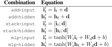
Table 1: Incorporation of doc2vec signal in the
decoder. d denotes the doc2vec vector; it (ht) is the input (hidden) vector at timet; and “[·;·]” denotes vector concatenation.
input, new context and new hidden state, respec-tively;∗is the elementwise vector product; andσ
is the sigmoid activation function.
Given an input word and previous hidden state, the decoder predicts the next word and generates the summary one word at a time.
To generate summaries that are related to the document, we incorporate thedoc2vecinput doc-ument signal to the decoder using several meth-ods proposed by Hoang et al. (2016). There are two layers where we can incorporatedoc2vec: in the input layer (input), or hidden layer (hidden). There are three methods of incorporation: addi-tion (add), stacking (stack), or via a multilayer perceptron (mlp). Table 1 illustrates the 6 possible approaches to incorporation.
Note that add requires doc2vec to have the
same vector dimensionality as the layer it is com-bined with, andstack-hiddendoubles the hidden
size (assuming they have the same dimensions), resulting in a large output projection matrix and longer training time.
4 Experiments and Results
4.1 Datasets
We test our decoupled architecture for the headline generation task. Following Chopra et al. (2016), we run experiments using GIGAWORD, DUC03
andDUC04.3
GIGAWORDis preprocessed according to Rush
et al. (2015), yielding 4.3 million examples. For in-domain experiments, we randomly sam-ple 2,000 examsam-ples for each validation and test set, and use the remaining examples for training. We tune hyparameters based on validation per-plexity and evaluate performance on the test set
3GIGAWORD: https://catalog.ldc.upenn.
edu/LDC2003T05;DUC:http://duc.nist.gov/
using the ROUGE metric (Lin, 2004), following the same evaluation style of benchmark systems (Rush et al., 2015; Chopra et al., 2016). For out-of-domain experiments, we use the same models trained from GIGAWORD, but tune using DUC03
and test onDUC04;DUC03 andDUC04 each have
500 examples.
For thedoc2vecencoder, we train using GIGA -WORD and infer document vectors for validation
and test examples using the trained model. Valid and test examples are excluded from thedoc2vec
training data.
4.2 Hyper-parameter tuning
For the encoder, we explore using a range of docu-ment lengths (first 20/30/40/50 words) to generate the input representation. Validation results show that using the first 20 words produces the best per-formance, suggesting that this length contains suf-ficient information to generate headlines.
We next test the 6 different ways to incorporate
doc2vec into the decoder. We find that stacking thedoc2vecvector with the input (stack-input) has the most consistent performance, whilemlpis
competitive, andaddperforms the worst. Interest-ingly, for mlpand stack, we find the difference betweeninputandhiddento be small.
For the recurrent decoder, hyper-parameters that are tuned include the mini-batch size, hidden layer size, number of LSTM layers, number of training epochs, learning rate, and drop out rate. The best results is achieved with a mini-batch size of 128, hidden size of 900, and one LSTM layer. The best perplexity is obtained after 3 to 4 epochs, with a learning rate of 0.001. More training epochs are needed when we reduce the learning rate to 0.0001. For in-domain experiments, the best re-sults are achieved with a dropout rate of 0.1, while for out-of-domain experiments, the best perfor-mance prefers a higher dropout rate at 0.4. This suggests that dropout plays an important role in combating over-fitting, and it is especially useful for out-of-domain data.
4.3 Results
We compare our model (RDS: Recurrent
De-coupled Summarizer) with 4 state-of-art models:
ABS, ABS+ (Rush et al., 2015); RAS-LSTM and
RAS-Elman (Chopra et al., 2016), which are all
System ROUGE-1 ROUGE-2 ROUGE-L
ABS 29.6 11.3 26.4
ABS+ 29.8 11.9 30.0
RAS-LSTM 32.6 14.7 30.0
RAS-Elman 33.8 16.0 31.2
RDS 30.7 11.3 27.6
RDS(75%) 29.1 10.0 26.3 RDS(50%) 27.4 8.9 24.9
Table 2: Comparison of ROUGE scores (full length F-score) for in-domain experiments.
System ROUGE-1 ROUGE-2 ROUGE-L
Prefix 22.4 6.5 19.7
ABS 26.6 7.1 22.1
ABS+ 28.2 8.5 23.8
RAS-LSTM 27.4 7.7 23.1
RAS-Elman 29.0 8.3 24.1
RDS 16.7 3.7 14.4
Table 3: Comparison of ROUGE scores (recall at 75 bytes) for out-of-domain experiments.
report ROUGE-1/2/L recall at 75 bytes in Table 3, where only the first 75 bytes of model-generated summary is used for evaluation against the refer-ences.
ABS employs an attentive encoder and a feed-forward neural network decoder. ABS+ works in
the same way as ABS, but further tunes the
de-coder using Z-MERT (Zaidan, 2009). RAS-LSTM
andRAS-Elmanare detailed in Section 2; the only difference between them is thatRAS-LSTMuses an
LSTM decoder, while RAS-Elman uses a simple RNN decoder. Prefixis a baseline model where the first 75 byte of the document is used as the title. Looking at Table 2, models with a recurrent de-coder (RDSandRAS) perform better than those with a feed-forward decoder (ABS). The decoupled
ar-chitectureRDSachieves competitive performance,
although the fully joint RAS models achieve the best results. Chopra et al. (2016) found that RAS models perform best with a beam size of 10, while we found thatRDSperforms best with greedy argmax decoding.
We further experiment with training RDS
us-ing less data (50% and 75%), and find that its performance degrades slightly. Encouragingly, its ROUGE-1 is comparable to ABS when RDSis
trained using only 75% of the training data, and it takes 2 days of training time (RDS) instead of 4 days (ABS).
I A North Korean man arrived in Seoul Wednes-day andsought asylumafter escaping his hunger-stricken homeland, government officials said. A North Korean manarrives in Seoul to seek asylum
for homeland security officials say. D North Korean mandefects toSouth Korea.
I King Norodom Sihanoukhasdeclinedrequests to chair a summit of Cambodia ’s toppolitical leaders, saying the meeting would not bring any progress in deadlocked negotiations to form a government . A King Sihanoukdeclinesto meet Cambodian leaders
on eve of talks with Cambodia.
D Cambodian king refusesto meet with leaders of political leaders.
I Former U.S. president Jimmy Carter , who seems a perennial Nobel peace prize also-ran ,could have wonthe coveted honor in 1978had it not been for strict deadline rules for nominations.
A Former U.S. president Jimmy Carterwinstop honor for Nobel peace prize nominations.
D CarterwinsNobel prize in literature.
Table 4: System generated article summaries. I: reference summary; A:RAS-Elman; and D:RDS.
For out-of-domain experiments, we compute ROUGE recall at 75 bytes and find thatRDS
per-forms poorly, even worse than the baseline method
Prefix. This suggests that the decoupled ar-chitecture is sensitive to domain differences, and highlights a potential downside of the architec-ture. Investigating methods that can improve cross-domain performance is a direction for future work.
5 Discussion and Conclusion
We present some summaries for DUC documents
generated by RAS-Elman and RDS in Table 4 to
better understand possible reasons for the poor in-domain performance of RDS. The first
obser-vation is the shorter headlines generated by RDS
compared to the DUC reference summaries and
RAS-Elman headlines. RDS headlines are short — at an average length of 8.13 — and this is due to the short length of GIGAWORD titles it
is trained on, at 8.50 words on average. On the other hand, the average length of DUC
refer-ence summaries andRAS-Elmanheadlines is 11.63 and 13.08 words respectively; this explains why
RAS-Elman achieves better performance, since a
longer sentence would have a better chance to score higher in ROUGE.
word matching, as is evidenced bySihanouk and Cambodian kingin the second example.4 Lastly, the bag-of-words view of thedoc2vecencoder re-sults in some meaning loss: in the third example, Jimmy Carterdid not actually win the Nobel peace prize, for example.
We also computed the source copy rate of the systems.5 We find that, on average, RDS copies only 50.7% of its predicted words from input doc-ument, whileABSandABS+copy at a rate of 85.4%
and 91.5%. This is interesting, as it suggests that it paraphrases more than other systems, while achieving similar ROUGE performance.
To summarise, we proposed decoupling the encoder–decoder architecture as is traditionally used in sequence-to-sequence problems. We tested the decoupled system on news title genera-tion, and found that it performed competitively in-domain. Out-of-domain experiments, however, re-veal sub-par performance, suggesting that the de-coupled architecture is susceptible to domain dif-ferences.
References
Sumit Chopra, Michael Auli, and Alexander M. Rush. 2016. Abstractive sentence summarization with at-tentive recurrent neural networks. InProceedings of the 2016 Conference of the North American Chap-ter of the Association for Computational Linguistics: Human Language Technologies, pages 93–98, San Diego, California, June. Association for Computa-tional Linguistics.
Jeffrey Elman. 1998. Generalization, simple recurrent networks, and the emergence of structure. In Pro-ceedings of the Twentieth Annual Conference of the Cognitive Science Society.
Cong Duy Vu Hoang, Trevor Cohn, and Gholamreza Haffari. 2016. Incorporating side information into recurrent neural network language models. In Pro-ceedings of the 2016 Conference of the North Amer-ican Chapter of the Association for Computational Linguistics: Human Language Technologies, pages 1250–1255, San Diego, California, June. Associa-tion for ComputaAssocia-tional Linguistics.
Sepp Hochreiter and J¨urgen Schmidhuber. 1997. Long short-term memory. Neural Computation, 9:1735– 1780.
4Informal manual evaluation forRDS,ABS,ABS+andRAS
on GIGAWORDreveals thatABS,ABS+andRASare also gen-erating words that are of similar meaning, and that overall, RDSis less prefered by annotators.
5Source copy rate is defined as the fraction of generated
words that are in the original source documents.
Jey Han Lau and Timothy Baldwin. 2016. An em-pirical evaluation of doc2vec with practical insights into document embedding generation. In Proceed-ings of the 1st Workshop on Representation Learn-ing for NLP, pages 78–86, Berlin, Germany, August. Association for Computational Linguistics.
Quoc V Le and Tomas Mikolov. 2014. Distributed representations of sentences and documents. In In-ternational Conference on Machine Learning, pages 1188–1196.
Chin-Yew Lin. 2004. Rouge: A package for auto-matic evaluation of summaries. In Stan Szpakowicz Marie-Francine Moens, editor, Text Summarization Branches Out: Proceedings of the ACL-04 Work-shop, pages 74–81, Barcelona, Spain, July. Associa-tion for ComputaAssocia-tional Linguistics.
Tomas Mikolov, Martin Karafi´at, Lukas Burget, Jan Cernock`y, and Sanjeev Khudanpur. 2010. Recur-rent neural network based language model. In Inter-speech, volume 2, page 3.
Tomas Mikolov, Ilya Sutskever, Kai Chen, Greg S Cor-rado, and Jeff Dean. 2013. Distributed representa-tions of words and phrases and their compositional-ity. InAdvances in Neural Information Processing Systems, pages 3111–3119.
Alexander M. Rush, Sumit Chopra, and Jason Weston. 2015. A neural attention model for abstractive sen-tence summarization. In Proceedings of the 2015 Conference on Empirical Methods in Natural Lan-guage Processing, pages 379–389, Lisbon, Portugal, September. Association for Computational Linguis-tics.