Improving forecast accuracy
Improving the baseline forecast for
cheese products
by use of statistical forecasting
Project name: Improving forecast accuracy Business Group: Cheese, Butter & Milk powder Project
manager:
Freek van Sommeren Discipline: Supply chain
Author: F. van Sommeren (Freek) Student number: s0198285
Principals: F. Knulst-Wouda (Francisca) J. Kroes (Jacob)
Version: Public Start date: 18/04/2011 Supervisors
University of Twente:
dr.ir. L.L.M. van der Wegen (Leo) dr. P.C. Schuur (Peter)
Course: Master Thesis IEM (194100060)
Sent to: Principals, Steering Group, University of Twente Location: Amersfoort
ABSTRACT
This master thesis project was carried out at the supply chain department of
FrieslandCampina Cheese. This research project, analyzes the applicability of statistical forecasting for cheese products. The project focuses on forecasts for baseline sales. Baseline sales are the sales that are left when promotion sales have been excluded. FrieslandCampina wants to use APO (a forecast module in SAP) to create statistical forecasts. In this research project, we explore the statistical models that are available in APO. Because APO cannot optimize the parameters for every statistical model, we create an advanced forecasting tool in Microsoft Excel to optimize the parameters per model. Our analysis indicates that implementation of statistical forecasting would benefit FrieslandCampina. Because of the great variety and amounts of products at
FrieslandCampina, we select 80 products to analyze in our research. 72,5% of these products show an improvement in forecast performance.
PREFACE
This master thesis is the final result of my master study Production and Logistic Management at the University of Twente. This thesis is the result of six months of research at the supply chain department of FrieslandCampina Cheese in Amersfoort. It has been an enriching experience, which contributed extensively to my professional and personal development.
First of all, I would like to thank my first supervisor at the University of Twente, Leo van der Wegen. I thank Leo for his critical feedback over the course of the entire project. His precise guidance and feedback have contributed greatly to the quality of this research project.
Secondly, I would like to thank my second supervisor at the University of Twente, Peter Schuur. I thank Peter for sharing his knowledge and his feedback.
I enjoyed working at the supply chain department at FrieslandCampina. Colleagues at FrieslandCampina were very friendly and helped me whenever necessary. I would especially like to thank Francisca Knulst-Wouda for giving me feedback and the flexibility to conduct my research. Another special thanks to Jacob Kroes for providing me with information and helping me whenever it was needed.
Furthermore, I would like to thank my family and friends for their support and the pleasant time I had as student in Enschede. I would especially like to thank my parents for giving me the opportunity to finish this study.
Lastly, I would like to thank my girlfriend, for the support and inspiration she has given me.
MANAGEMENT SUMMARY
Problem
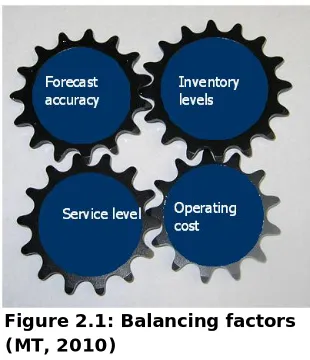
The supply chain department is charged with finding the right balance between operating costs and service and inventory levels. To create the right balance between the three factors, service level, inventory level, and operating costs, forecasts should be accurate. Underestimation of demand can result in lost sales, dissatisfied customers, or insufficient resources for production. Overestimation of demand can result in high operating costs and high inventory.
The supply chain and sales departments are dissatisfied with the current forecast method. FrieslandCampina presumes a more accurate forecast to be important for the increase of service levels and the decrease of inventory levels and operating costs. FrieslandCampina wants to improve the performance of Cheese & Cheese Specialties with regard to delivery to customers in balance with working capital. In order to achieve optimal performance from the working capital, the forecast accuracy needs to be improved.
FrieslandCampina wants to increase forecast accuracy by using statistical forecasting. However, it is unclear whether statistical forecasting is the appropriate method. Furthermore, it is unclear which statistical forecast models exist and which forecast models can be used.
Analysis
By interviewing sales planners and project managers, we identified various causes for the current forecast inaccuracy. The following causes were identified:
1. Inaccurate forecast procedure
2. Inaccurate use of performance evaluation 3. Insufficient use of system functionalities in APO
Our project focuses on the insufficient use of system functionalities. We want to increase forecast performance by using the statistical forecast functionality in APO. This master thesis project focuses on the applicability of statistical forecasting for the portfolio of FrieslandCampina.
Results
We created eight groups of articles, which cover all of FrieslandCampina’s markets. We created three groups in the branded retail market, two groups in the non-branded retail market, and three groups divided over the B2B, IM, and indirect markets. Furthermore, the group division is based on sales volume per article, importance of customer, and variance in demand.
performance when statistical forecasting is used. Statistical forecasting decreases the forecast performance for products with strongly fluctuating sales patterns or products with an unpredictable intermittent sales pattern.
This master thesis project explores several statistical forecast models. The best model and parameters vary greatly per product. The damped trend model is the best statistical model for 26,3% of the products and the simple exponential smoothing model is the best statistical model for 20% of the products.
Recommendations
The implementation of statistical forecasting results in an improvement of the forecast performance. To implement statistical forecasting, we provide FrieslandCampina with several recommendations.
Model and parameter selection
The forecast module APO can automatically select the appropriate statistical forecast model and optimize its parameters. This function requires three years of data. At this point, one and a half years of data is available. Therefore, we cannot automatically select the optimal model.
In this project, we created an advanced forecast tool in Microsoft Excel to select the best model and its optimal parameters. FrieslandCampina can use this forecast tool to select the best model and its parameters for the complete portfolio of FrieslandCampina. This requires a lot of work. Therefore, we advise FrieslandCampina to use the simple or double exponential smoothing model in APO. The parameters for these two models can be optimized by APO. We discovered that there is a 1,4% decrease in forecast accuracy and a 3,27% decrease in forecast bias performance when we use the best of the simple or double exponential smoothing model instead of the overall best model. We advise FrieslandCampina to use the double exponential smoothing model when dealing with a (damped) trend in the sales pattern of the product, and to use the simple exponential smoothing model when there is no trend.
When three years of data are available, we advise FrieslandCampina to use the automatic model selection function in APO.
Aggregation levels
In Section 7.2, we analyze which aggregation level should be used in each case. We advise FrieslandCampina to forecast production on the basic material/age level (in case age is older than 10 weeks) and to forecast packaging on the commercial article level.
Outlier method
In Section 5.1, we describe the modified z-score method to statistically remove outliers from the sales pattern. We use the modified z-score method because the parameters used to calculate the modified z-score are minimally affected by outliers. APO does not contain the modified z-score method but does contain the median method. The median method calculates the median over the level-value and the median over the trend-value from past data. Based on these two median values, a tolerance lane is calculated. Values outside the tolerance lane are outliers.
Forward buying effect
In this master thesis project we also analyzed the forward buying effect. The forward buying effect is the loss of sales after a promotion. Our analysis indicates that the forward buying effect takes place in the first two weeks after a promotion. We analyzed the quantity of the forward buying effect in the first two weeks. On average, there is a 30,5% decrease in sales in the first two weeks after a promotion.
The forward buying effect varies greatly between promotions. In some cases, the forward buying effect shows an 80% decrease in sales. In other cases, there is an increase in sales after a promotion. Therefore, it is difficult for FrieslandCampina to incorporate the forward buying effect.
We advise FrieslandCampina to do more research on the forward buying effect.
Tracking signal
The sales patterns of products can change over time. Therefore, it is possible for the statistical forecast model and parameters to no longer be appropriate. To control the model and parameters, we advise FrieslandCampina to use Trigg’s tracking signal. This tracking signal indicates when a forecast is out of control and the parameters need to be updated. A tracking signal indicates if the forecast is consistently biased high or low. The tracking signal should be recomputed each period. The movement of the tracking signal is compared to the control limits; as long as the tracking signal is within these limits, the forecast is under control. Trigg’s tracking signal is available in APO.
Demand forecasting versus sales forecasting
The data we use in our research is based on actual sales. When sales are lost due to incorrect forecasting or capacity problems, we do not fulfill the complete sales orders from customers. Therefore, the actual sales are not equal to the demand. When we make forecasts based on actual sales, we do not incorporate the complete demand and the forecasts will be incorrect.
Therefore, we advise basing forecasts on actual demand instead of actual sales.
Improved forecast process
We created an improved forecast process (see Figure 7.9 in Section 7.6). The forecast process incorporates all the steps that are required to statistical forecast products, including a new planning strategy per product and the forecast module APO to create statistical forecasts. We advise to use the improved forecast process.
TABLE OF CONTENTS
Abstract
iii
Preface
iv
Management summary
v
Table of contents
viii
1. Introduction
1
2. Research approach
5
2.1
Problem identification
5
2.2
Project objective
6
2.3
Problem statement
6
2.4
Research questions
6
2.5
Scope of the project
8
2.6
Deliverables
8
3. Current situation
9
3.1
Product characteristics
9
3.2
Market characteristics
10
3.3
Supply chain department
13
3.4
Analysis
16
4
.Literature research
19
4.1
Sales pattern components
19
4.2
Moving averages and smoothing methods
20
4.3
Other methods
23
4.4
Forecast models used in other food organizations
25
4.5
Forecast measures
26
5. Model selection method
28
5.1
Cleaning historic data
28
5.2
Model selection method
30
6. Statistical forecast performance
35
6.1
Article selection
35
6.2
Statistical forecasting vs. current forecast method
36
6.3
Conclusion forecast performance
45
6.4
Coefficient of variation boundary
47
6.5
Best model and parameters
47
7. Implementation
50
7.1
APO implementation
50
7.2
Aggregation levels
51
7.3
Forward buying effect
52
7.4
Control mechanism
54
7.5
Managing products
55
7.6
Improved forecast process
57
8. Conclusions and recommendations
60
8.1
Recommendations
61
8.2
Suggestions for future research
62
1.
INTRODUCTION
In the framework of my master program Industrial Engineering and Management, I performed a master thesis project at the company, FrieslandCampina. This chapter describes the company at which my research took place. FrieslandCampina wants to increase their forecast accuracy by introducing statistical forecasting. In Chapter 2, the research problem, the research approach, and the structure of this report are described in more detail.
1.1 Company introduction
Royal FrieslandCampina is a multinational dairy company, fully owned by the dairy co-operative Zuivelcoöperatie FrieslandCampina, which is comprised of 15,326 dairy farms in the Netherlands, Germany, and Belgium. Daily FrieslandCampina provides food for hundreds of millions of people all over the world. Products are sold in more than one hundred countries, the key regions being Europe, Asia, and Africa. In 2010, sales amounted to nearly 8.2 billion Euros. FrieslandCampina employs over 20.000 employees, in 25 countries. See Figure 1.1 for more company facts.
Figure 1.1: Company facts (www.frieslandcampina.com, 2011)
FrieslandCampina is deeply rooted in the culture and commerce of the Netherlands, Germany, and Belgium. FrieslandCampina is a global company, but focuses on local communities and customers. The company is also deeply rooted in many countries outside Europe.
1.2 History
In late December 2008, the merger of Friesland Foods and Campina, two companies that developed along similar lines, results in the creation of FrieslandCampina. It all started in the 1870s, when, all over the Netherlands, farmers joined forces in local co-operative dairy factories. They did this to safeguard the sales of their milk (without the benefit of modern refrigeration they had to work together) and to gain more power on the market.
Groningen and Drenthe, and Coberco covers Gelderland and Overijssel. In the west of the Netherlands, several co-operatives merged into Melkunie Holland in 1979. Melkunie Holland also acquired several privately owned dairy companies. 1979 is also the year that DMV Campina was established in the south. DMV Campina and Melkunie Holland merged into Campina Melkunie in 1989. In 1997 four major co-operatives in the north and east of the Netherlands merged to create Friesland Coberco, which later became Friesland Foods. In 2001, Campina merged with the Milchwerke Köln/Wuppertal co-operative from Cologne, Germany and the De Verbroedering co-operative from the Antwerp region of Belgium. This created the international Campina co-operative.
In December 2007, Friesland Foods and Campina announced their intentions to merge. One year later, in December 2008, they received the approval of the European competition authorities to become FrieslandCampina.
1.3 Strategy
FrieslandCampina’s strategy is to increase their added value. At the same time, they want to ensure that all the milk produced by the cooperative’s member dairy farmers reaches its full value. To this end, FrieslandCampina formulated route2020; a new strategy aimed at achieving accelerated growth in selected markets and product categories.
In developing and expanding their value, FrieslandCampina primarily focuses on growth, profitability, and milk valorization (adding value to milk). The route2020 strategy defines six value drivers to achieve value growth.
Worldwide growth in dairy-based beverages by increasing the share in total consumption.
Strengthening market positions in infant nutrition, both ingredients and end products, worldwide.
Increased market share in branded cheese, by, for example, expanding the brand portfolio.
Geographical growth in the above categories and improving the strong positions outside of these categories.
Foodservice in Europe: strengthening and expanding existing strong positions in the eating-out category, partly through geographical expansion.
Strengthening of basic products such as standard ingredients, industrial cheese, and private labels, in order to reduce the share of member milk that is processed into commodities.
1.4 Products and locations
FrieslandCampina processes over 10 billion kilograms of milk per year in consumer products such as dairy drinks, baby and infant food, cheese, butter, cream and desserts, and butter and cream products to professional customers. Aside from that, FrieslandCampina processes ingredients and components for the food and pharmaceutical sectors. These products are primarily sold in 25 countries, located mainly in Europe, Asia, North America, and Africa, while the ingredients are sold worldwide. FrieslandCampina carries leading brands, including Appelsientje, Best Cool, Chocomel, Campina Milner and Mona.
dairy-based beverages, infant and toddler nutrition, cheese, butter, cream, desserts and functional dairy-based ingredients.
FrieslandCampina has limited product presence in America, but the continent is still important to the company, especially to the operating companies which sell high quality dairy ingredients. FrieslandCampina DMV, FrieslandCampina Domo, and FrieslandCampina Creamy Creation all have sales offices in the United States.
FrieslandCampina can be found all over Europe, where 70% of its total turnover is generated. In Europe, there is a broad product range, extending from daily fresh liquid milk to cheese, butter, and fruit juice. FrieslandCampina’s ingredients, which vary from milkshake mixes to caseinates, are used by professional and industrial food producers all over Europe to prepare their products. FrieslandCampina has its own sales outlets in many European countries. Aside from that, there are also production plants throughout Europe, mainly in the Netherlands, Germany, and Belgium. This is not surprising, since FrieslandCampina dairy cooperative member farmers are based in these three countries. In many African and Middle Eastern countries, FrieslandCampina sells products that are tailored to local conditions. These include large amounts of condensed milk and milk powder, as well as cheese and butter. Peak and Rainbow are well-known FrieslandCampina brands that are sold in these countries.
FrieslandCampina is a key player in the dairy sector in Africa and the Middle East, which accounts for 10% of the company’s total sales. There are also outlets in Nigeria and Saudi Arabia. Many of the products, which are sold in Africa and the Middle East, are based on milk supplied by FrieslandCampina’s own member farmers in the Netherlands, Germany, and Belgium. FrieslandCampina Creamy Creation is also active on the African market, where it sells cream liqueur in sachets.
FrieslandCampina has a long history on the Asian market. The company has, for example, been selling dairy products in Vietnam and Indonesia for more than 80 years. This initially began with the sale of sweetened condensed milk and has since extended to a wide range of dairy products. Whether it is milk-based drinks, baby food, yoghurts, yoghurt drinks, or advanced dairy ingredients, FrieslandCampina’s products can be found in many Asian countries. There are also sales offices and production plants across Asia. Asia accounts for 17% of the company’s total turnover.
1.5 Organization
In order to be successful on the market, FrieslandCampina must have a keen eye for customer wishes and connect these to the potential uses of milk. This is what FrieslandCampina’s operating companies do every day. These operating companies are active in specific product groups, and sometimes also in a specific country or region (see Figure 1.2).
Each of the four business groups stands for a certain product group;
• Consumer Products Europe (milk, dairy drinks, cream, coffee creamers, yoghurts and desserts in Western Europe);
• Consumer Products International (milk, milk powder, condensed milk, yoghurts and desserts in Eastern Europe, Asia and Africa);
• Cheese and Butter (cheese and butter, worldwide);
• Ingredients (ingredients for the food and pharmaceutical industry, worldwide).
The departments of the Corporate Center are engaged in Business Group-overarching strategic issues. These include contact with the member dairy farmers.
Figure 1.2: Organization of the company (www.frieslandcampina.com, 2011)
1.6 Business Group
Our project focuses on the Business Group Cheese, Butter & Milk Powder. The Business Group produces and sells a broad range of cheeses, butters, and milk powders. In Europe, FrieslandCampina’s butter is sold under the familiar brands by other dairy producers such as Campina (Botergoud and Buttergold), Landliebe, and Milli. In countries outside Europe FrieslandCampina sells consumer-packaged butter and butter oil under brand names such as Campina and Frico.
2.
RESEARCH APPROACH
This chapter introduces the project assignment. Based on the method of Heerkens et al. (2004), the core problem is identified. After the identification of the core problem, this chapter describes the research approach.
2.1 Problem identification
Before discussing our project, the core problem must be identified (Heerkens, 2004). The core problem is the main problem, which needs to be solved in this project. To identify our core problem, different managers of the Business Group Cheese, Butter, and Milk Powder were interviewed. During the interviews with these managers, who all work for the supply chain department or the sales department, we discovered cohesion between the problems that were mentioned.
The supply chain department is charged with finding the right balance between operating costs, service level, and inventory level. In order to create the right balance between the three factors, service level, inventory level, and operating costs, forecasts must be accurate (see Figure 2.1). Underestimating demand can result in lost sales, dissatisfied customers and insufficient resources. Overestimating demand can result in high operating costs and a high inventory.
Planning decisions for Cheese & Cheese Specialties products are based on forecasts. According to Silver et al. (1998), planning decisions and inventory management could be steered by effective
forecasting. Effective forecasting is essential to achieve service levels, to plan allocation of total inventory investment, to identify needs for additional production capacity, and to choose between alternative operating strategies. The problem is, however, that it is improbable for forecasts to be 100% correct. By choosing the right forecast method and achieving the most accurate forecast possible, the total expected relevant costs for decisions should be as low as possible.
The supply chain and sales departments are dissatisfied with the current forecast method. FrieslandCampina presumes a more accurate forecast is important to increase service levels, decrease inventory levels, and operating costs. Currently FrieslandCampina has difficulty achieving forecast accuracy1 targets. In 2010, the forecast targets2 were not achieved for most markets. The actual forecast accuracy deviates on average -5,5% compared to the forecast accuracy targets.
FrieslandCampina wants to improve the performance of Cheese & Cheese Specialties with regard to delivery performance to customers, in balance with working capital. To create optimal performance from working capital, the forecast accuracy needs to be improved.
Therefore, we identified the following core problem.
1 Forecast accuracy: 100% - MAPE (see Section 4.5) 2
[image:13.595.356.511.282.462.2]Forecast targets for the complete demand (baseline and promotions)
Core problem:
The current forecast method results in insufficient forecast accuracy.
2.2 Project objective
The management team of the supply chain department Cheese & Cheese Specialties wants to improve forecast accuracy. Currently, the forecast applies to complete demand3.
We are going to analyze the usefulness of statistical forecasting for the baseline demand4. The overall forecast framework from Silver et al. (1998) suggests a forecasting system where statistical forecasting is involved. By means of statistical forecasting, we want to increase baseline forecast accuracy.
We are going to analyze the use of statistical forecasting per product per market. If statistical forecasting seems to be appropriate, different statistical forecast models will be analyzed concerning accuracy and bias.
FrieslandCampina intends to use the software tool APO (planning component of SAP) to generate forecasts. We are going to explore if the standard models in SAP are appropriate to forecast the products sold by FrieslandCampina.
Forecast error reduction is a main goal for this project. As stated earlier, the increase of forecast accuracy leads to decreasing inventory levels, operating costs, or increasing service levels. These factors are not performance measures for this project. The project focuses fully on increasing forecast accuracy.
2.3 Problem statement
The core problem concerns insufficient forecast accuracy. FrieslandCampina wants to increase forecast accuracy by using statistical forecasting. However, it is unclear whether statistical forecasting is the appropriate method. Furthermore, it is unclear which statistical forecast models exist and which forecast models would best fit to the demand patterns at FrieslandCampina.
The following problem statement captures the above described assignment:
Is statistical forecasting an appropriate method to forecast the baseline demand for Cheese and Cheese Specialties products and, if so, which statistical forecast models does FrieslandCampina need to use for cheese products to improve their baseline forecast accuracy?
2.4 Research questions
To solve the problem, research questions need to be defined. To execute this research, the scientific approach towards the design of a new forecasting process from DeLurgio (1998) is used (see Appendix B). This is an effective approach and provides attention to detail (DeLurgio, 1998). The first steps used inthis scientific approach will be followed. Within the various steps, research questions need to be answered.
3 Complete demand: demand including promotions
4 Baseline demand: demand that will be sold without support of any specific action (e.g.
Chapter 2: Research approach
Chapter 2 of this report contains the first step in the approach from DeLurgio. This section contains the identification, the objective, the problem statement, and the research approach of this project.
Chapter 3: Current situation
The Business Group FrieslandCampina Cheese, Butter, and Milk Powder has a broad range of products. This project focuses on cheese products. FrieslandCampina is present within a number of markets. Per product level, the different types of markets need to be analyzed, in order to identify the characteristics of each market. Interviews with project managers, sales planners and account managers will allow us to analyze the current situation and identify causes for the currently insufficient forecast accuracy.
Therefore, the following research questions are set up.
1. What are the characteristics per product per market at FrieslandCampina? 2. How are forecast processes organized and controlled in the current situation? 3. What are the causes for the low forecast performance?
Chapter 4: Literature research
The next step in DeLurgios approach is formulating statistical models. To create a starting point, literature, more accurately, literature on quantitative forecast models, will be researched in order to find statistical forecast models. To create statistical forecast models, FrieslandCampina needs to know how the performance of these models can be measured. In literature, we will search for methods to measure the accuracy of different models.
4. Which statistical forecast models are used in other (food) organizations? 5. How can the forecast performance be measured?
Chapter 5: Data cleaning and model selection method
After researching the literature, we will explore how the historical data needs to be cleaned to create an accurate baseline demand. All peaks caused by promotions and push orders will be removed from historic data. In this chapter, we will also design a model selection method to obtain the best forecast models for FrieslandCampina.
6. How should historical data be cleaned to create statistical baseline forecast models?
7. How should FrieslandCampina select the best appropriate statistical model to forecast each product?
Chapter 6: Performance evaluation
8. Which statistical forecast models would fit best to the demand patterns at FrieslandCampina?
9. Which products at FrieslandCampina are appropriate for using statistical forecasting?
Chapter 7: Implementation
At this point, we will explore how to implement statistical forecasting into APO. There are models present in APO, but not all parameters for each model can be optimized. We will analyze how to handle these difficulties. We will also advise FrieslandCampina on the management of the forecast per product and review the forecast process. Therefore, the following research questions are setup:
10.How can FrieslandCampina implement statistical forecasting?
11.How should FrieslandCampina manage the forecast of their products? 12.What should the new forecast process look like?
2.5 Scope of the project
FrieslandCampina’s current forecast method develops two different types of forecasts: baseline forecast (sales under normal circumstances) and promotion forecast (extra sales due to promotions). According to FrieslandCampina, promotions cannot be forecasted statistically because promotions fluctuate heavily and are often ordered by customers. Therefore, we focus our research on the baseline forecast.
This master thesis project only focuses on baseline forecast for existing products. Hence, forecasts for product introductions are excluded. This project focuses on regular sales without dump sales or sales due to oversupply.
Furthermore, not all products from FrieslandCampina are taken into account. The project focuses on cheese products, all other products are excluded from analysis.
Not all cheeses will be analyzed. During project execution, a representative group of products will be chosen in cooperation with FrieslandCampina.
This project only explores quantitative forecast models, qualitative forecast models will be explored by FrieslandCampina.
2.6 Deliverables
We create an advisory report concerning the usefulness of statistical forecasting for the products sold by FrieslandCampina. This report contains:
Analysis of current forecast method
Description of useful statistical forecast models Description of useful forecast measures
Advice about best fit statistical forecast models
Advice on which markets are appropriate for using statistical forecasting Advice about the creation of the baseline demand
Advice about the best forecast aggregation level Control mechanism for statistical models
3.
CURRENT SITUATION
In this chapter, we describe the current forecast process used by FrieslandCampina. Because each forecast process is different per market, we first describe product characteristics in Section 3.1 and market characteristics in Section 3.2. Secondly, we present overviews of production, planning and forecasting processes in the current situation in Section 3.3. Finally, in Section 3.4, we analyze causes for the insufficient forecast accuracy in the current situation.
3.1 Product characteristics
FrieslandCampina produces 130 different cheeses, currently using twelve factories, located throughout the Netherlands and Germany. They produce two types of products; nature cheese and rindless cheese. Nature cheese matures in the open air, where the quality of air is regulated. In the production of this type of cheese, a special coating for natural moistening is used, which is the original approach for producing cheese. The rindless cheese matures in closed plastic and does not get a coating. In most cases, rindless cheese is used for industrial purposes, while nature cheese is used for direct consumption. Popular nature cheeses are Gouda, Milner, Edam, and Maasdam.
Another characteristic of cheese is the age of the product. Cheese matures over time, maturation time depends on the cheese recipe. Nature cheese can be matured up to a year. Rindless cheese can be matured up to a few weeks. The third and fourth characteristics are weight and commercial product appearance.
3.1.1 Product aggregation levels
In Chapter 6, we test statistical forecasting for different aggregation levels. Therefore, we first identify the different levels. FrieslandCampina distinguishes seven product aggregation levels for cheese products. The aggregation levels are the following:
Brand
Brand is the highest aggregation level of products. Every specific brand has its own characteristics that belong to their specific type of cheese. Typical brands produced by FrieslandCampina are: Milner, Frico, Old Dutch Master and Slankie.
Cheese variety
Cheese variety is a group of basic materials from the same brand, which have the same structure or weight. Cheese varieties from the Edam ball are: baby Edam, Edam ball 1,9 kg, Edam ball, and special Edam ball.
Basic material
Basic material is the aggregation level that shows which ingredients, model and size are used for a specific cheese. The basic material level is used by production planning to plan the production of cheeses. Basic materials from the special Edam ball are: Edam 1,9 kg NL Veg, Edam Tkr 1,9 kg NL, Edam Sambal 1,9 kg NL, Edam Rooksmaak 1,9 kg NL and Kaas 20+ 1,9 kg Bolvorm ELF DV.
Age
Aggregation level age is used to specify the maturation time of the cheese. The Goudse Wielen 12 kg can be matured for: 15 days, 4 weeks, 7 weeks, 11 weeks, 13 weeks or 17 weeks.
Cutting code
The cutting code specifies how the cheese is sliced into pieces. Example cutting codes are: 510 (wheels), 210 (wedges), 310 (flat pieces) or 410 (blocks).
Commercial article
The level below cutting code is the commercial article level. A customer places an order based on commercial article. The order desk translates this into the, at that moment, correct, valid logistic material, i.e., commercial article level and logistic material level are on same aggregation level, The difference being, that a logistic material contains more information.
Logistic material
All data is saved on the logistic material level. This level provides information about the customer (is connected with planning customer, see Section 3.3.2), the product appearance (bill of material), the age, the basic material, the cheese variety and the brand. This is the article planned upon and packed, transported and delivered to a customer.
All products below the basic material aggregation level could be moved to another type of product, e.g., in case there is a shortage in 11 week cheese for the Edam 1,9 kg, we could choose to mature a 7 week cheese for the Edam 1,9 kg a little longer and let it mature for 11 weeks.
3.2 Market characteristics
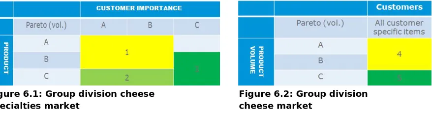
We start by explaining the direct sector. The direct channels can be divided into Business-to-Business (B2B), customers and retail customers. The B2B market is about selling rindless cheese to industry customers, such as grated cheese for Dr. Oetker. The retail channel is about direct marketing towards retail customers, such as Albert Heijn and Aldi. The retail market can be subdivided into two markets; branded and non-branded. Branded cheese is called the cheese specialties market and non-branded cheese is called the cheese market.
FrieslandCampina considers the production of cheese its core business. For some products, FrieslandCampina controls the entire process, from buying the raw materials, up to the sale of final products to customers. For other products, FrieslandCampina outsources different stages of the process. For example, FrieslandCampina outsources the maturation, packaging, and trade process of cheese. Processes can be outsourced to two types of customers from the indirect sector. First, customers that take over the maturation process and/or packaging process and trade process are called Value Added Resellers (VARs). Second, customers that only take over the trade process, which are called trade customers, and sell their products mainly to small shops and markets. Aside from the indirect market, products are also exported. Exporting products signifies the sale of products to international markets (markets outside the EU). Export, therefore, is also referred to as the International Markets.
Figure 3.2: FrieslandCampina Cheese markets
3.2.1 Demand characteristics
[image:19.595.152.448.349.621.2]Within the non-branded retail market, demand is characterized by numerous contracts with customers. This is called a contract-driven business. New contracts are obtained through a bidding process called tendering. New tenders are usually confirmed approximately three months before the start of a contract. Several products in the indirect, B2B and International Markets are make-to-order products or packed-to-order products. Make-to-order products are produced on order. Packed-to-order products are produced on forecast and packed on order. The indirect, B2B, and international markets are also contract-driven businesses.
All markets are equally important to FrieslandCampina and will be included in the performance evaluation for statistical forecasting (Chapter 6).
3.2.2 Customer aggregation levels
Just as we analyze statistical forecasting on different product aggregation levels, we also analyze statistical forecasting on different customer aggregation levels. We distinguish three customer aggregation levels.
Figure 3.5: Customer aggregation levels
Distribution channel
The highest aggregation level is the distribution channel. This level describes the market to which the customers belong. The distribution channel can be subdivided into five different channels, namely, International Markets, Branded Retail Europe, Non-Branded Retail Europe, Business-to-Business, and Indirect.
Reporting customer
The reporting customer is a purchase organization for a number of planning customers. The purchase organization Bijeen, for example, purchases goods for Jumbo Group Holding and Schuitema.
Planning customer
The planning customer can be subdivided into different distribution centers (DC’s). Because promotions by customers are planned on planning customer level, description on DC level is not relevant to our research.
3.3 Supply chain department
This section provides an overview of the production and planning process and its relation to the forecast process.
FrieslandCampina has twelve production locations, which are all located in the Netherlands. The supply chain department is a bridge between the sales department and these production locations. Using forecasting and the limits of production capacities and the milk supply, the supply chain department decides on the quantity and allocation that are to be produced each week. Milk supply can be seen as an important constraint on cheese production. The milk quantity needed to produce cheese in a particular week has to be aligned by the milk supply for that specific week by the corporate department of Milk Valorization.
3.3.1 Production and planning overview
The production plants are managed by the planning department, centrally located in Amersfoort. Production planning and packaging planning depend on forecasting. The forecast process will be explained in the next section.
Production is scheduled every week, and one week after scheduling, basic materials are produced at production plants.
The produced products leave the chain at different stages (Figure 3.6). The first group of products leaves the chain immediately after production; these products are called exit-factory products (EF). The second group leaves after the maturation facility; these are the large-packaged items (LPI). The third group of articles is transported to a specialized packaging facility where it is packed into small-packaged items (SPI). The number of different articles increases and the volume of the entire flow decreases towards the end of the chain.
Figure 3.6: Production and planning overview
Production
customers. These products are called the ‘ex-factory’ stream and account for roughly twenty percent of the total sales volume. In official terms, ‘Ex-factory’ is also referred to as ‘Ex-works’, a trade term requiring the seller to deliver goods at his or her own place of business. All other transportation costs and risks are assumed by the buyer.
Maturation
After fifteen days of storage at the production plants, the cheese is transported to a specialized maturation facility. At the maturation facility large volumes of cheese are stored until they are ready to be sold.
In a maturation facility the cheese is stored for two to sixty weeks, depending on the commercial age of the end product. The commercial age is the official ripening age, which is communicated to the customer.
Packaging
Two weeks before products are packed, the packaging forecast is determined. The packaging forecast is compared with the production forecast from a few weeks earlier. Oversupplies or shortages in the production forecast can be solved by using age tolerance. Age tolerance means that the ripening period of a specific cheese type can be used variably. For example, the norm for the Milner Licht Gerijpt is to ripe nine weeks. To solve oversupplies or shortages in cheese demand, the cheese could be packed in week eight (lower tolerance), or in week eleven (upper tolerance). Age tolerance is applied when there is not enough cheese available in the norm age.
If necessary, the cheese of week eleven could be cooled for a maximum of four weeks. Therefore, it has a maximum internal shelf life of four weeks. During cooling, the ripening process is severely slowed down. This can be used as a solution in case of very disappointing demands. This solution is only used in emergency cases.
Cheeses are packed, either in large or in small items. The LPIs are packed at a maturation facility. After the LPIs are packed, they leave the production chain and are transported to a distribution center or sold directly to a customer (Figure 3.6). The packaging type of the large packaged items is different, for example, a carton box, a plastic crate, cut in halves, coated with paraffin, etcetera. Not every facility can pack every type of packaging shape. The SPIs are packed at a specialized packaging facility elsewhere. A small part of the small packaging activities is outsourced to specialized packaging companies. After packaging, some products are sold directly to the customer (PTO5-products), while other products are sent to a warehousing and distribution center where customer orders are handled. These products are delivered on customer demand (PTS6-products).
3.3.2 Forecast overview
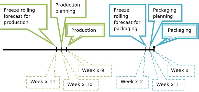
Production planning and packaging planning depend on forecasting. The forecast is determined by the sales planner and the sales team by creating a rolling sales forecast, starting eighteen months before production. The rolling forecast is updated weekly and is forecast on customer level and logistic material level. The same rolling forecast is used for the production planning and the packaging planning. Two weeks before the production of the cheese starts, the rolling forecast is frozen on the basis material/age
5 PTO: Pack-to-Order 6
level and is used to steer production planning. The production forecast is made on the basic material/age aggregation level (see Section 3.1.1). Figure 3.7 shows the forecast timeline for cheese that needs to ripen for nine weeks. If the cheese needs to ripen for nine weeks, the forecast horizon for production needs to be eleven weeks. If the cheese needs to ripen for 26 weeks, the forecast horizon for production needs to be 28 weeks. After a number of weeks (which depends on the commercial age of the cheese), the rolling forecast is frozen on the commercial article level to steer packaging planning. The packaging forecast is made on the commercial article aggregation level (see Section 3.1.1). This rolling forecast is frozen two weeks before packaging.
Figure 3.7: Forecast timeline for nine-week cheese
The forecast process is supported by the system APO (Advanced Planner and Optimizer). This is a forecast module from the ERP-system SAP. The forecast process starts with loading the actual sales from last year into APO. The sales planner makes manual adjustments in forecast after consulting the account manager. Account management is accountable for final forecast and has final control over the goods that will be produced. FrieslandCampina distinguishes five types of markets, namely retail (branded and non-branded), indirect, B2B and international markets. Per market, there is difference in forecast method. The following three subsections give a description of forecast characteristics per market.
Retail
The retail market can be subdivided into two markets; branded market and non-branded market. The branded market is mainly a promo-driven business and the non-branded market is a contract-driven business.
The forecast for the non-branded market is based on the continuation of current contracts. Expectations for gaining new contracts through tendering are not taken into account. New tenders are not included in the forecast because of the uncertainty involved in obtaining the contract.
For the non-branded market, forecasts for promotions are only included on customer indication. There are no production reservations for optional promotions. The sales manager indicates what amounts are produced when, in case of promotions.
The rolling forecast is evaluated every two weeks. These evaluations are discussed by the sales team and, if necessary, the forecast is adapted.
Promotions play an important part in forecasts for the branded cheese market, and are followed in detail. The promotion forecast is steered by the sales team in consultation
with the customers. The baseline forecast is a process that runs parallel to the promotion forecast. The first step in creating the baseline forecast is uploading the actual sales from the previous year. Then, the sales planner, in consultation with the account manager, makes manual adjustments. Promotion forecast is then added to this baseline forecast. The account manager makes estimations for the promotion demand in consultation with some customers. Not all customers announce their promotions. Estimations for promotion demand are added to the baseline forecast. Promotion effects from history are stored in separate files, without a link to APO. These historic effects are used to estimate the effects of future promotions.
Indirect
Within the indirect market the sales planner creates a rolling forecast, starting 18 months before production. The rolling forecast is updated weekly and is forecast on customer level and item level. Fixed contracts are the most important information upon which the baseline forecast is based. Expected contracts are used for baseline adjustment. Long-term forecasting (18 months before production) is generated by assuming the extension of current contracts. The sales planner creates a forecast in cooperation with the sales manager by use of APO. The sales manager is responsible for expectations regarding future contracts.
In the indirect market sales orders are used for many products’ short-term forecasts. When this is the case, no forecast is made since the forecast registered in APO will be overwritten by the customer orders.
Business-to-Business and International Markets
The forecast process for B2B and international markets is based mainly on the forecast process for the indirect market, but there are small differences. The contracts are the main information for sales forecast. The problem, however, is that this information is not always available to the sales planner. Although the contract information is the focus of the forecast process, the sales planner does not always have access to this information. For short-term forecasting, the forecast should be based on information on actual customer orders. Another difference in the forecast process for B2B, compared to the process within the indirect market, is that product orders are not always received in time and translated into SAP. Furthermore, the short-term forecast is not always overwritten by customer orders.
3.4 Analysis
FrieslandCampina has problems reaching forecast accuracy targets7. In 2010 the forecast targets were not achieved for most markets (see Appendix A). After interviewing sales planners and project managers, we have concluded that the current forecast method can be improved. We identified various causes for the current forecast inaccuracy. The following causes were identified:
1. Inaccurate forecast procedure
2. Inaccurate use of performance evaluation
3. Insufficient use of system functionalities
7
The following three subsections provide more details about the causes of the current forecast inaccuracy.
3.4.1 Inaccurate forecast procedure
There is no distinction between forecast generation and forecast enrichment (i.e. forecast evaluation). Sales planners spend a lot of time creating new forecasts. Section 3.3 describes how sales planners load the actual sales from last year into the forecast system. The sales planner makes manual adjustments for all products every two weeks. These manual adjustments need to be discussed with the account manager. This process applies only to sales under normal circumstances. There are also promotions that need to be taken into account. These promotions must also be discussed with the account manager. This entire forecast process generates a lot of work, leaving no time to evaluate the forecast. In conclusion, the dominance of the administrative aspect of the sales planner’s function does not allow him to use forecast enrichment. Every day, sales planners work with demand patterns for their product group and obtain market intelligence from these patterns. Because too much time is spent generating new forecasts, no time is left to add market intelligence.
Furthermore, forecast procedures lack standardization . Each market has its own sales planners and every sales planner has his own forecast procedure. Sales planner’s roles and responsibilities are not standardized. Every sales planner has his own method for generating forecasts. Sales planners’ responsibilities vary greatly from person to person, depending on his experience and the attitude of the account team.
3.4.2 Inaccurate use of performance evaluation
KPIs are calculated every week (periodic review) to measure forecast accuracy (e.g. the mean absolute percentage error). These KPIs only measure the short term forecast. There are no KPIs for mid- and long-term forecasts. The second problem is that the forecast bias performance is not properly used in periodic reviews. Yet another problem is that the KPIs used in short-term forecasts are interpreted in different ways. Furthermore, the weekly forecast performance is only reported in the total forecast, which includes promotion forecasting. This complicates the analysis of the baseline forecast performance.
The last problem is that the measured forecast performance is not followed up by actions. The forecast performance is measured each week, but the sales planner does not perform any actions based on these forecast performances or may not have time to do this.
3.4.3 Insufficient use of system functionalities
Sales planners make use of APO (Advanced Planner and Optimizer), which is a forecast module in SAP. APO can create a forecast using several methods. Appendix C shows the models that are available in APO. The sales manager uses the ‘copy history’ method in APO. This means that the historical sales data from the previous year is copied (i.e. naïve method). There are more appropriate statistical forecast methods available in APO. APO contains statistical forecasting methods like the Linear Regression Method and the Holt-Winters method. The sales planner does not use these methods. For more functionalities in APO, visit http://help.sap.com. Sales planners do not make use of statistical forecast methods and therefore do not use all APO’s system functionalities.
4.
LITERATURE RESEARCH
In this chapter we research literature on sales pattern components (Section 4.1), statistical forecast models (Section 4.2, 4.3 and 4.4) and forecast measures (Section 4.5). We start by explaining the sales pattern components.
4.1 Sales pattern components
According to DeLurgio (1998), the most common methods of statistical forecasting make estimates of the future on the basis of past patterns. In this research we will explore univariate forecast methods. Univariate forecast methods are based on one variable, without using relations to other variables. Univariate forecast methods are based on demand patterns from history. All forecast methods described in this section are extrapolative. Extrapolative forecast methods are based on the assumption that a certain demand pattern from the past will persist in the future. Because of this assumption, extrapolative methods only use historical values as input for their forecast models. Sales patterns can be divided into five components:
level, trend, seasonal variations, cyclical movements and irregular random fluctuations (Silver et al., 1998). When there is only one level present in a sales pattern the series is constant through time. Trend specifies the rate of growth or decline of a pattern over time. Seasonal variations are periodic and recurrent patterns, which result from natural forces or arise from human decisions or customs. Cyclical variations are the result of the business cycles that are the result of economic activity. In time series analysis, irregular fluctuations are the residues that remain after the effects of the other four components have been identified and removed from the time series. These fluctuations are the result of unpredictable events.
Using these concepts we can formulate the following model:
Demand in period t = (Level) + (Trend) + (Seasonal) + (Cyclic) + (Irregular)
This report concentrates on short- to medium-term forecasting and will therefore not incorporate cyclical effects (Silver et al., 1998).
We describe models that have the following patterns:
=
+
(level pattern)
=
+
+
(trend pattern)
= ( +
)
+
(trend-seasonal pattern)
Figure 4.2: trend pattern
0 30 60 90 120 150 180
0 5 10 15 20 25 30 35
Figure 4.4: Cyclical pattern
0 30 60 90 120 150 180
0 5 10 15 20 25 30 35
Figure 4.3: Seasonal pattern
0 30 60 90 120 150 180
0 5 10 15 20 25 30 35
Figure 4.1: level pattern
0 30 60 90 120 150 180
where
= demand in period t = level
= trend
= a seasonal coefficient appropriate for period t
= independent random variable with mean 0 and constant variance
4.2 Moving averages and smoothing methods
We will start by explaining moving average and smoothing forecasting models.
4.2.1 Simple moving average
According to Silver et al. (1998), the simple moving average is appropriate when demand displays only a level pattern.
The simple N-period moving average, at the end of period t, is given by;
̅
,= ( +
+
+
. . +
)/
[4.1]
In this case the letters x represent actual demand in the corresponding periods. The forecast for period
+
(= , ) is then:,
=
̅
,If there is a change in the parameter , a small value of N is preferable because it gives more weight to recent data, and thus picks up changes more quickly. Typical N values that are used range from 3 to as high as 12.
4.2.2 Weighted moving averages
It is normally true that the immediate past is most relevant in forecasting the immediate future. For this reason, weighted moving averages place more weight on the most recent observations. The simple moving average uses equal weights for each observation, but a weighted moving average uses different weights for each observation. The only restriction on the weights is that their sum equals one. An advantage of the weighted moving average is that the weights placed on past demands can be varied. See the following formula for an example of a four-period weighted moving average;
,
= 0.1
∗
+
0.2
∗
+ 0.3
∗
+ 0.4
∗
)
[4.2]
When using a moving average, it is difficult to determine the optimal number of periods to include in the average. However, this is not a problem for exponential smoothing.
4.2.3 Simple exponential smoothing
According to Silver et al. (1997) simple exponential smoothing is probably the most widely used statistical method for short-term forecasting. The basic underlying demand pattern assumes the level model.
=
+ (1
−
)
=
ℎ
=
[4.3]
,
=
,
=
ℎ
,
ℎ
,
ℎ
+
4.2.4 Exponential smoothing for a trend model
The model described in Subsection 4.2.3 is based on a model without a trend and is therefore inappropriate when the underlying demand pattern contains a significant trend. When this is the case, exponential smoothing for a trend model is needed. The basic underlying model is the trend model:
=
+
+
Holt (1957) suggests a procedure that is a natural extension of simple exponential smoothing:
=
+ (1
−
)(
+
)
[4.4]
=
(
−
) + (1
−
)
=
Where and are smoothing constants and, the difference
−
is an estimate of the actual trend in period t.=
To estimate the forecast at end of period t the following formula should be used:
,
=
+
,
=
ℎ
,
ℎ
,
ℎ
+
Double exponential smoothing
DeLurgio (1998) describes Brown’s double exponential smoothing method to compute the difference between single and double smoothed values as a measure of trend. It adds this value to the single smoothed value together with adjustment for the current trend. It uses a single coefficient, alpha, for both smoothing operations.
Brown’s model is implemented with the following equations (
′
denotes a single smoothed and"
denotes the double smoothed value):′
=
+ (1
−
)
′
" =
′
+ (1
−
) "
= 2
′ −
"
=
(
−
" )
[4.5]
,
=
+
Exponential smoothing with damped trend
Sometimes data is so noisy, or the trend so erratic, that a linear trend is not very accurate. Gardner & McKenzie (1985) introduced a damped trend procedure that works well in these situations.
They recommend using the following formulas:
=
+ (1
−
)(
+
)
=
(
−
) + (1
−
)
[4.6]
,
=
+
,
=
ℎ
,
ℎ
,
ℎ
+
where is a dampening parameter. If = 1, the trend is linear and identical to the normal exponential smoothing with trend model. If = 0 the method is identical to standard simple exponential smoothing. In case the dampening parameter is such that 0 < < 1, the trend is damped.
4.2.5 Exponential smoothing procedure for a seasonal model
There are a number of products in organizations that exhibit demand patterns that contain significant seasonality. Seasonal series result from events that are periodic and recurrent (e.g. monthly changes recurring each year). Common seasonal influences are climate, human habits, holidays, and so on. The underlying model in this case is:
= ( +
)
+
Winters (1960) suggest the following procedure, which is a natural extension of the Holt procedure described in Subsection 4.2.4. The parameters are updated according to the following three equations:
=
(
) + (1
−
)(
+
)
=
(
−
) + (1
−
)
[4.7]
=
+
(1
−
)
=
,
= (
+
)
,
=
ℎ
,
ℎ
,
ℎ
+
where , and are smoothing constants lying between 0 and 1. Silver et al. (1998) suggests the use of a search experiment to establish reasonable values for the smoothing constants.
4.2.6 Evaluation
Makridakis et al. (1993) used 1001 time series to compare the accuracy of several methods. When data is deseasonalized and exponential smoothing methods are compared to sophisticated forecast procedures, in some cases, they perform the same. Furthermore, the research identified that when randomness in data increases, it is preferable to select simple forecast procedures.
Murdick and Georgoff (1986) present general characteristics of short-range through long-range forecasting methods. The effective horizon lengths of methods are longer as we move from univariate, to multivariate8, to qualitative methods. Our research focuses on univariate methods. We can assert that, in general, short-horizon forecasts are typically more accurate than longer-horizon forecasts. The forecast accuracy of the simple exponential smoothing method is high9 when the horizon length remains under one month (DeLurgio, 1998). The single exponential smoothing method performs worse as the forecast horizon increases because the method does not take trends into consideration. Forecast accuracy for more complex smoothing methods, like trend or seasonal models, is high9 when the horizon length remains under three months. For complex smoothing methods, medium9 forecast accuracy is obtained when the forecast
horizon length is between three months and three years.
4.3 Other methods
The methods that have been described so far are moving average or smoothing methods. There are a number of other methods that could also be appropriate for the products sold by FrieslandCampina. The following methods could be appropriate:
4.3.1 Simple linear regression
The simple linear regression model assumes that demand is a linear function of time:
=
+
+
A least squares criterion is used to estimate values, denoted by and , of the parameters and . The resulting modelled value of , denoted , is then given by
=
+
If there are n historical observations, then the least squares criterion involves the selection of and to minimize the sum of the squares of the n differences between and . That is (Silver, Pike, & Peterson, 1998),
=
(
−
−
)
Using calculus we can show that
8
Multivariate: analysis of more than one statistical variable
9 The term high, medium, and low refers to the relative accuracy of methods. No
=
∑
−
(
+ 1
2 )
∑
(
−
1)/12
and
=
/
−
( + 1)/2
Once the parameters and are estimated, the following model can be used to forecast demand in a future period:
,
=
+
[4.8]
4.3.2 Croston’s method
The exponential smoothing forecast methods described earlier have been found to be ineffective where transactions occur on an infrequent basis. Croston’s method could be appropriate when dealing with intermittent demand. Croston’s method makes separate exponential smoothing estimates of the average size of a demand and the average interval between demands. The method updates the estimates after demand occurs; if a review period t has no demand, the method just increments the number of time periods since the last demand. The method uses the following formulas (Willemain et al., 1994):
= 0
" = "
" = "
=
+ 1
" = "
+ (
−
"
)
" = "
+ (
−
"
)
= 1
=
" =
" =
=
" =
=
ℎ
Combining the estimates for demand and interval provides the estimate for the mean demand per period:
" =
""
[4.9]
These estimates are only updated when demand occurs. When demand occurs in every review interval, Croston’s method is identical to simple exponential smoothing.
4.3.3 Box- Jenkins method
The stochastic variations in the demand models that we have considered in the aforementioned models are assumed to be independent. This is a major simplification. It is easy to imagine situations where this is not the case. When dealing with only a small number of large customers, it is to be expected that demands in consecutive periods will sometimes be negatively correlated. A high demand in one period can indicate that several of the customers have replenished their supplies, and that it is reasonable to expect demand in the next period to be somewhat lower. However, situations also exist where demand is correlated positively. A high demand in one period may mean that the product has been exposed to more potential customers, and that demand can be expected to be high again in the next period. Forecasting techniques that can handle correlated stochastic demand variations and other more general demand processes have been developed by Box and Jenkins (1970). The models proposed by Box and Jenkins are more complex than either simple regression models or exponential smoothing procedures.
4.4 Forecast models used in other food organizations
Some industries and companies are affected by cyclical fluctuations in the economy (or other environmental factors). Forecasting cyclical changes is difficult, as the length and depth of cycles vary - sometimes considerably. Makridakis (1986) claims that companies in anti-cyclical industries, such as the food and medical industry, can rely on quantitative forecast methods. FrieslandCampina focuses on the food industry, so quantitative models could be appropriate for the company.
Miller et al. (1991) researched food production forecasting through simple time series models. In their study, they explored simple models with minimal data sto