Munich Personal RePEc Archive
A consumption-based approach to
exchange rate predictability
Ojeda-Joya, Jair
Banco de la Republica
24 May 2019
Online at
https://mpra.ub.uni-muenchen.de/94231/
A CONSUMPTION-BASED APPROACH TO
EXCHANGE RATE PREDICTABILITY
Jair N. Ojeda-Joya
*We study whether the implications of an international consumption-based asset-pricing model are useful to provide out-sample predictability evidence for the real exchange rate. This model implies a predictability equation that results from the presence of both internal and external consumption habits in the utility function. In this equation, domestic, U.S. and world consumption growth are predictors of the real exchange rate. Our empirical exercises confirm this connection by providing evidence of short-term predictability on the bilateral rates of 15 out of 17 countries vis-à-vis the U.S. over the post Bretton-Woods float. A non-linear GMM estimation of some parameters of the model also brings about evidence of the presence of consumption habits in the utility function.
JEL C53, F31, F47, G15
Keywords: exchange rates, out-of-sample, predictability, asset pricing, habits
1. INTRODUCTION
This paper provides a framework to study exchange rate predictability by developing a
consumption-based asset-pricing model that includes internal and external habit formation2.
Within this model, it is possible to show that the presence of habits in consumers’
preferences implies that the exchange rate has a predictable component which depends on
past consumption growth3. That is, if we combine the first order condition for optimal
consumption-savings allocation with an international arbitrage condition, it is possible to
derive a forecasting equation for the exchange rate due to the presence of habits in the utility
function. We estimate this forecasting equation with both linear and non-linear econometric
methods using data for 17 industrialized economies over the Post-Bretton-Woods float. We
find significant evidence of short-run out-of-sample predictability in 14 countries by
computing tests that compare the forecasting power of the model with a random-walk
forecast, a regularly used benchmark for evaluating exchange rate models (Rossi, 2013).
We interpret the empirical results in the context of a consumption-based asset-pricing model
with N economies, complete markets, imperfect international risk sharing and representative
consumers whose preferences include internal and external habit persistence. The economic
reason for Real Exchange Rate (RER) predictability in this framework is the habit effect of
past consumption growth on current marginal utility and thus on the stochastic discount
factors (SDFs) that domestic and foreign investors use to value financial assets. In this
framework, the difference between external and domestic SDFs drives RER variations.
As a robustness check for these predictability results, we attempt to measure the degree of
habit persistence and its relative importance across countries by estimating the relevant
parameters of the utility function using non-linear GMM methods. Results from this
estimation show significant and strong habit effects in 15 out of the 17 economies under
study.
2 In this paper, external habits are very similar to the definition of catching up with the Joneses in Abel (1990) but within an open-economy interpretation. This approach is conceptually similar to that in Campbell and Cochrane (1999) but with a different specification in the utility function.
3
This paper relates to the empirical literature on exchange rate determination models. In
particular, the problem has some similarities to the one originally described by Meese and
Rogoff (1983) about the poor out-of-sample forecasting power of the monetary approach to
exchange rate determination.Several papers have shown that alternative specifications of the
monetary model have out-of-sample predictability power for long-run horizons (one year or
more); see for example, Mark (1995), Mark and Sul (2001), Groen (2005), Engel et al (2007),
and Cerra and Saxena (2010).
Additionally, a few papers show out-of-sample predictability evidence with alternative
exchange rate models. Gourinchas and Rey (2007) study an international financial
adjustment model in which RER changes are the result of disequilibria of the country’s
external accounts. Molodtsova and Papell (2009), Byrne et al (2016), Ince et al (2016) among
others estimate forecasting equations derived from Taylor-rule specifications for monetary
policy in each country. Rogoff and Stavrakeva (2008) perform robustness exercises
comparing alternative models and conclude that the out-of-sample predictability evidence is
still weak on horizons shorter than one year. One possible reason for this weakness is that
the intensity of the relation between exchange rates and alternative fundamentals is time
varying. Sarno and Valente (2009) and Fratzscher et al (2015) show the evidence and
propose “scapegoat” models based on time-varying elasticities. Rossi (2013) surveys this
literature and concludes that the most promising models are those based on Taylor rules or
external accounts4.
The current paper presents a forecasting equation derived from a consumption-based
asset-pricing model and shows that it has interesting predictability properties on the
one-quarter-ahead horizon. An important difference with previous works on exchange rate predictability
is that the model has only implications for the (bilateral) RER. A possible caveat of this
approach is that its main predictor is household consumption a quarterly national-accounts
variable, which makes it difficult to perform monthly forecast exercises as in most of the
literature on the topic.
Backus et al (2001) initiated the use of consumption-based asset pricing models to study the
necessary conditions to solve the forward premium puzzle. Lustig and Verdelhan (2007)
empirically show that low interest rate currencies provide investors with a hedge against
consumption-growth risk, which explains the uncovered interest rate parity puzzle.
Verdelhan (2010) presents an asset-pricing model with external consumption habits that
reproduces the countercyclical risk premium and the observed relation between exchange
rates and consumption growth. We partially follow Verdelhan’s (2010) approach to derive an exchange rate predictability equation based on consumption data.
The outline of the paper is the following. Section 2 describes the consumption-based
asset-pricing framework and its implied forecasting equation for the RER. Section 3 presents the
econometrics methods for out-of-sample predictability evaluation. Sections 4 and 5 present
results for each country and for alternative forecasting windows, respectively. Section 6
presents the in-sample non-linear estimation of the most relevant parameters of the model.
Finally, Section 7 concludes.
2. A CONSUMPTION-BASED ASSET-PRICING MODEL
2.1. Basic Framework
The following consumption-based asset-pricing framework is based on Abel (1990, 2008)
but it is extended to include N countries (𝑖 = 1,2, … 𝑁). The representative consumer in each
country 𝑖 maximizes:
𝑈𝑖,𝑡= 𝐸𝑡[∑∞𝑗=0𝛽𝑗(1−𝛼1 ) (𝐶𝑉𝑖,𝑡+𝑗
𝑖,𝑡+𝑗𝛾𝑖 )
1−𝛼
] (1)
In Equation (1), 𝛼 denotes the risk aversion coefficient, 𝛽 is the time discount factor, 𝐶𝑖,𝑡 is
the level of household consumption in each country5 and 𝑉
𝑖,𝑡𝛾𝑖 is the benchmark level of
consumption where the parameter 𝛾𝑖 measures the degree of habit persistence in country i.
5𝐶
Benchmark consumption includes past domestic consumption as well as past world
consumption:
𝑉𝑖,𝑡 = [(𝐶𝑖,𝑡−1)𝐷(𝐶𝑤,𝑡−1)1−𝐷] (2)
In Equation (2), 𝐶𝑤 denotes world consumption and D is a weight that measures the
importance of domestic consumption relative to world consumption in the composition of
the benchmark level of consumption. World consumption is the geometric weighted average
of consumption across countries. The weights 𝜔𝑖 in Equation (3) are determined by the
relative economic size of country 𝑖.
𝐶𝑤= ∏𝑁𝑖=1𝐶𝑖𝜔𝑖 (3)
The utility framework in Equations (1) to (3) nests the standard CRRA case when 𝛾 = 0,
since in this case benchmark consumption does not have any influence in utility. When 𝛾 >
0 instead, utility depends on the ratio between domestic and benchmark consumptions. The
presence of 𝑉𝑡𝛾 in the utility function captures both internal and external habit formation. We
interpret external habits as the satisfaction from consuming as much as the average world
level of consumption or more.
From Equation (1), it is possible to compute the marginal utility of consumption in each
country.
𝜕𝑈𝑖,𝑡
𝜕𝐶𝑖,𝑡 =
1 𝐶𝑖,𝑡𝐸𝑡[(
𝐶𝑖,𝑡
𝑉𝑖,𝑡𝛾𝑖) 1−𝛼
− 𝛾𝑖𝐷𝛽 (𝐶𝑉𝑖,𝑡+1
𝑖,𝑡+1𝛾𝑖 )
1−𝛼
] (4)
Notice that marginal utility in (4) when 𝛾𝑖 = 0, is exactly equal to the case of a standard
CRRA utility function (𝐶𝑖,𝑡−𝛼). Therefore, it is possible to partition Equation (4) into three
components: standard CRRA, benchmark consumption and habits. We specify these three
components in Equation (5).
𝜕𝑈𝑖,𝑡
𝜕𝐶𝑖,𝑡 = 𝐶𝑖,𝑡
−𝛼𝑉
The component 𝐶𝑖,𝑡−𝛼is the standard CRRA marginal utility which decreases with current
consumption and with the risk-aversion degree (𝛼). The effect of benchmark consumption
is measured by 𝑉𝑖,𝑡𝛾𝑖(𝛼−1). Notice that, as long as there is some habit persistence (𝛾𝑖 > 0), the
effect of benchmark consumption on marginal utility is positive only if there is enough risk
aversion (𝛼 > 1). If there is not any habit persistence or in the log-utility case (𝛼 = 1), benchmark consumption has not any effect on marginal utility.
Equation (6) defines the component 𝐻𝑖,𝑡 that measures the effect of internal habits on
marginal utility. When there are no internal habits in the utility function, 𝐻𝑖,𝑡 = 1. Otherwise,
𝐻𝑖,𝑡 is a fraction that considers the fact that a higher consumption today increases the
benchmark level of consumption and thus decreases tomorrow’s utility. We assume that the
parameters of the model are such that 𝐻𝑖,𝑡> 0, and therefore marginal utility, is strictly
positive.
𝐻𝑖,𝑡 = 1 − 𝛽𝐷𝛾𝑖𝐸𝑡(𝑋𝑖,𝑡+11−𝛼)𝑋𝑖,𝑡𝐷𝛾𝑖(𝛼−1)𝑋𝑤,𝑡(1−𝐷)𝛾𝑖(𝛼−1) (6)
In Equation (5), 𝑋𝑖,𝑡corresponds to the gross rate of consumption. Therefore, we define:
𝑋𝑖,𝑡+1= 𝐶𝑖,𝑡+1⁄𝐶𝑖,𝑡 and 𝑋𝑤,𝑡+1= 𝐶𝑤,𝑡+1⁄𝐶𝑤,𝑡.
Equation (5) and the definition of benchmark consumption allow us easily computing the
Stochastic Discount Factor (SDF) or pricing kernel, as the product of the time discount
factor (𝛽) and marginal utility growth, see Equation (7).
𝑀𝑖,𝑡+1 = 𝛽𝑋𝑖,𝑡+1−𝛼 𝑋𝑖,𝑡𝐷𝛾𝑖(𝛼−1)𝑋𝑤,𝑡(1−𝐷)𝛾𝑖(𝛼−1)(𝐻𝐻𝑖,𝑡+1𝑖,𝑡 ). (7)
2.2. Implications for the Real Exchange Rate
We describe the relation between exchange rates and SDFs following the asset-pricing
of one price, there exists a unique SDF in the space of traded assets. Lustig and Verdelhan
(2007) derive a similar result and apply it to the cross-section of foreign currency risk.
Let 𝑀𝑢𝑠,𝑡+1 denote the SDF of US investors. 𝑄𝑡is the real exchange rate (RER) expressed as
US goods per foreign good, therefore, if 𝑄𝑡 decreases then the real US dollar appreciates. All
investors have access to a foreign-currency return 𝑅𝑖,𝑡+1. Equations (8) and (9) are the Euler
conditions for US and foreign investors, respectively:
𝐸𝑡(𝑀𝑖,𝑡+1𝑅𝑖,𝑡+1) = 1 (8)
𝐸𝑡(𝑀us,𝑡+1𝑅𝑖,𝑡+1𝑄𝑡+1⁄ ) = 1 𝑄𝑡 (9)
The uniqueness of the SDF in the space of traded assets and Equations (8) and (9) imply the
following relationship:
𝑀𝑖,𝑡+1 = 𝑀𝑢𝑠,𝑡+1𝑄𝑡+1⁄𝑄𝑡 (10)
Computing natural logarithms on both sides of Equation (10) we obtain:
𝑞𝑡+1− 𝑞𝑡 = 𝑚𝑖,𝑡+1− 𝑚𝑢𝑠,𝑡+1. (11)
Throughout this paper, lower case letters stand for the natural logarithm of the original
variables. In Equation (11), 𝑚𝑢𝑠,𝑡+1, 𝑚𝑖,𝑡+1are the US and country i’s log SDFs, respectively.
This equation implies that the log variation in the real exchange rate is equal to the difference
between the log SDFs across countries. Computing logs on both sides of (7) and inserting
this result in (11), we obtain the following expression for the real exchange rate as a function
of consumption growth and habit persistence in both countries:
∆𝑞𝑖,𝑡+1= −𝛼(𝑥𝑖,𝑡+1− 𝑥𝑢𝑠,𝑡+1) + 𝐷𝛾𝑖(𝛼 − 1)𝑥𝑖,𝑡− 𝐷𝛾𝑢𝑠(𝛼 − 1)𝑥𝑢𝑠,𝑡+
(1 − 𝐷)(𝛼 − 1)(𝛾𝑖− 𝛾𝑢𝑠)𝑥𝑤,𝑡+ ∆ℎ𝑖,𝑡+1+ ∆ℎ𝑢𝑠,𝑡+1 (12)
In Equation (12), growth rates for the RER and the habit effect are denoted ∆𝑞𝑖,𝑡+1 and
∆ℎ𝑖,𝑡+1, respectively. Notice that we interpret (12) as a forecasting equation in which changes
in the real exchange rate are determined by lagged values of domestic, US and world
implications for asset pricing through its effects on the marginal utility of consumption and
thus on SDFs.
There are two necessary conditions for predictability in Equation (12). First, the risk aversion
coefficient 𝛼 should be different from one; otherwise, the RER becomes neutral to the
presence of habit persistence. Second, we need 𝛾𝑖 ≠ 𝛾𝑈𝑆 for the exchange rate to be
predictable via the external habit channel.
2.3. Computing a Linear Forecasting Equation
To estimate the expected value of (12) using a linear regression framework, we use a
first-order Taylor approximation to ℎ𝑖,𝑡 and ℎ𝑢𝑠,𝑡 since both expressions are nonlinear functions
of consumption growth. For this approximation, we define the following:
𝓏𝑖,𝑡 ≡ 𝐷𝛾𝑖(𝛼 − 1)𝑥𝑖,𝑡+ (1 − 𝐷)𝛾𝑖(𝛼 − 1)𝑥𝑤,𝑡 (13)
Therefore, inserting (13) in (6) and taking logs, we can write ℎ𝑡 in the following simplified
way:
ℎ𝑖,𝑡 ≡ log(𝐻𝑖,𝑡) = log (1 − 𝐷𝛾𝑖𝛽𝐸(𝑋𝑖,𝑡+11−𝛼)ℯ𝑧𝑖,𝑡) (14)
Once we compute the derivative of (14), it is possible to express the first-order Taylor
approximation to ℎ𝑖,𝑡 around 𝐸(𝓏𝑖,𝑡) ≡ 𝓏̅𝑖 in the following way:
ℎ𝑖,𝑡 ≈ log(1 − 𝐷𝛾𝑖𝛽𝐸(𝑋𝑖,𝑡+11−𝛼)ℯ̅̅̅𝒵𝑖) − 𝐷𝛾𝑖𝛽𝐸(𝑋𝑖,𝑡+11−𝛼)ℯ𝒵𝑖̅̅̅
1−𝐷𝛾𝑖𝛽𝐸(𝑋𝑖,𝑡+11−𝛼)ℯ𝒵𝑖̅̅̅(𝓏𝑖,𝑡− 𝓏̅𝑖) (15)
From (15), we can compute ∆ℎ𝑖,𝑡+1 which consists of a constant multiplied by ∆𝑧𝑖,𝑡+1.
Therefore, using (13) and (15), we can calculate the expected value of ∆ℎ𝑖,𝑡+1, conditional on
information through t, in the following way:
In Equation (16),𝜃𝑖 is a constant parameter:
𝜃𝑖 ≡ 𝐷𝛾𝑖𝛽𝐸(𝑋𝑖
1−𝛼)ℯ𝒵𝑖̅̅̅
1−𝐷𝛾𝑖𝛽𝐸(𝑋𝑖1−𝛼)ℯ𝒵𝑖̅̅̅ (17)
Equation (16) also assumes a log normal distribution for consumption growth in all countries such that in each period t: log(𝑋𝑖,𝑡) ≡ 𝑥𝑖,𝑡~𝑁(𝑔, 𝜎2) (18)
Using (12), (16) and (18), it is possible to derive a linear forecasting equation for the expected variation of the real exchange rate as a function of past consumption growth in the domestic country, the US and the World: 𝐸𝑡(∆𝑞𝑖,𝑡+1) = 𝜓𝑖,0+ 𝜓𝑖,1∆𝐶𝑖,𝑡+ 𝜓𝑖,2∆𝐶𝑢𝑠,𝑡+ 𝜓𝑖,3∆𝐶𝑤,𝑡 (19)
The coefficients to estimate in Equation (19) are 𝜓𝑖,0, 𝜓𝑖,1, 𝜓𝑖,2 and 𝜓𝑖,3. These are functions of the deep parameters of the model: 𝜓𝑖,0 = (𝛼 − 1)𝑔(𝜃𝑢𝑠𝛾𝑢𝑠− 𝜃𝑖𝛾𝑖), (20)
𝜓𝑖,1= (1 + 𝜃𝑖)𝐷(𝛼 − 1)𝛾𝑖 (21)
𝜓𝑖,2= (1 + 𝜃𝑢𝑠)𝐷(𝛼 − 1)𝛾𝑢𝑠 (22)
𝜓𝑖,3= (1 − 𝐷)(𝛼 − 1)(𝛾𝑖(1 + 𝜃𝑖) − 𝛾𝑢𝑠(1 + 𝜃𝑢𝑠)) (23)
Notice that the sign of the coefficients 𝜓𝑖,0 and 𝜓𝑖,3 is determined by the relative size of the
parameters 𝛾𝑖 and 𝛾𝑢𝑠. Furthermore, 𝜓𝑖,1 and 𝜓𝑖,2 remain different from zero if there is a
positive degree of internal habits (𝐷 > 0). Additionally, under a sufficiently high-risk
aversion coefficient, 𝛼 > 1, we should expect a positive sign for 𝜓𝑖,1 and a negative sign for
3. DATA AND ECONOMETRIC METHODS: OUT-OF-SAMPLE
PREDICTABILITY TESTS
3.1 Data Description
Data consists of quarterly real exchange rates (RERs) and real household consumption for
18 advanced economies including the United States (US). We correct for seasonality by
computing annual variations of the natural logarithm of these variables. Bilateral RER data
are calculated with the consumer price index (CPI) and the average official exchange rate
with respect to the US dollar for each country. We retrieve these data from the International
Monetary Fund’s (IMF) International Financial Statistics (IFS). We use the following formula:
𝑞𝑖,𝑡= 𝑒𝑖,𝑡− 𝑝𝑢𝑠,𝑡+ 𝑝𝑖,𝑡 (24)
𝑞𝑖,𝑡 is the log RER, 𝑒𝑖,𝑡 is the log nominal exchange rate and 𝑝𝑖,𝑡 corresponds to the log CPI
for country i. An increase of the RER, according to this definition, corresponds to a real
appreciation of the currency vis-à-vis the US dollar. For countries in the European Monetary
Union (EMU), we only work with their previous currency before entering the union. In the
case of Germany, we only work with data from western Germany before the 1990
unification. For the remaining economies, all data are updated through 2015q26.
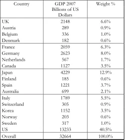
We construct real consumption with the nominal series on households’ consumption of
non-durable goods and services for each country. We deflate these series with CPI data, and
compute world consumption as described in Equation (3) and using the weights described in
Table A1 in the Appendix.
6
3.2. Three Alternative Tests
Following Rogoff and Stavrakeva (2008), we compute three alternative tests for
out-of-sample predictability power: Theil’s U (TU), Diebold-Mariano-West (DMW) and Clark-West
(CW). When the mean-square forecasting error is significantly smaller than the implied by a
random-walk model without drift, we regard it as a good forecast. This criterion has been
widely used in the exchange rate predictability literature since Meese and Rogoff (1983), and
it is still the toughest benchmark for any exchange rate model (Rossi, 2013).
The first step on the out-of-sample predictability exercise consists of choosing a forecasting
window. We initially use a 40-observation window to estimate Equation (19) with quarterly
data. Thus, in countries where the total sample spans 1973 q1 through 2015 q3, (173
observations), the forecasting window has approximately 133 observations. The second step
consists of using rolling regressions, with 40 observations each, to estimate the parameters in
Equation (19). Then we use these estimations to perform forecasts of exchange rates
one-quarter ahead. The final step is comparing the resulting 133 forecasts with actual real
exchange rate data and using these forecast errors to compute predictability tests.
Assume that 𝑦𝑡= 𝑞𝑡− 𝑞𝑡−1, is the quarterly variation of the real exchange rate. Let 𝑋𝑡 be the
matrix that includes the explanatory variables defined in Equation (19) and let 𝜓 be the
corresponding vector of constant coefficients. We are interested in comparing the
forecasting power of the model in Equation (19) with a random walk without drift. This
benchmark model implies: 𝑦𝑡 = 𝑒1,𝑡. We can rewrite the structural model in (19) as: 𝑦𝑡 =
𝑋𝑡−1𝜓 + 𝑒2,𝑡. Innovations terms 𝑒1,𝑡 and 𝑒2,𝑡 are assumed to be unobservable.
The estimated forecasts for the random walk and the structural model are 𝑦̂,𝑡+1= 0, and
𝑦̂2,𝑡+1= 𝑋𝑡𝜓̂𝑡 respectively, where 𝜓̂𝑡 is the least-squares estimator of 𝜓𝑡. The corresponding
forecast errors are 𝑒̂1,𝑡 and 𝑒̂2,𝑡, respectively. The Mean Squared Forecast Error (MSFE) for
either of the forecasting models is:
In Equation (25), P is the number of forecasts, T is the sample length and R is the
number of observations used to estimate 𝜓𝑡 on the first forecast. We define the TU test in
Equation (26) as the root square of the ratio between the MSFE of the structural model and
the random-walk model. Therefore, if TU is significantly lower than 1, the structural model
outperforms the random-walk model.
𝑇𝑈 = √𝑀𝑆𝐹𝐸2⁄𝑀𝑆𝐹𝐸1. (26)
The DMW test measures the difference between the MSFE of the random walk model and
that of the structural model (Equation 27). Therefore, a significant and positive DMW test
implies that the structural model outperforms the random walk.
𝐷𝑀𝑊 = 𝑀𝑆𝐹𝐸1− 𝑀𝑆𝐹𝐸2 (27)
The literature on forecasting has identified that both statistics, TU and DMW, tend to
over-reject the structural model when used to compare projections from nested models like those
in the current exercise7. In view of this problem, Clark and West (2006, 2007) propose a test
statistic (CW) which builds on the DMW test but takes into account that both models are
nested by assuming that, under the null hypothesis, the exchange rate follows a random walk.
Therefore, the null hypothesis in the CW test is computed under the assumption that the
population parameter vector is 𝜓 = 0, and that the forecast innovation terms are equal
across models: 𝑒1,𝑡= 𝑒2,𝑡.
𝑑̂ = 2𝑃−1∑𝑇𝑡=𝑅+1(𝑦𝑡+1𝑋𝑡𝜓̂𝑡) (28)
Clark and West (2006) show that if 𝑑̂, the quantity defined in (28), is significantly greater than zero, then the structural model outperforms the random walk. Therefore, the CW test
is defined in (29) as a significance test for 𝑑̂ where Ω𝑑̂is its estimated variance.
𝐶𝑊 = 𝑃√Ω0.5𝑑̂𝑑̂ (29)
7
We follow Rogoff and Stavrakeva (2008) by computing all three tests (TU, DMW and CW),
when performing out-of-sample predictability exercises, and by using bootstrapped critical
values in order to correct for the potential size distortion which results from working with
nested models.
3.3. Bootstrap Procedure
We use a non-parametric bootstrap procedure to calculate the p-values for the TU and
DMW tests, following Mark and Sul (2001). The real exchange rate behaves as a random
walk, according to the null hypothesis. For quarterly consumption growth, we fit Equation
(30) using least squares, to estimate its autoregressive structure and its correlation with the
real exchange rate.
∆𝐶𝑡𝑖 = 𝛿0+ ∑𝑑𝑘=1𝛿𝑘𝑦𝑡−𝑘+ ∑𝑙𝑘=1𝜁𝑘∆𝐶𝑡−𝑘𝑖 + 𝜀𝑡𝑖 (30)
In (30), we select the number of lags, d and l as well as the appropriate trend (constant or
linear), by minimizing a Bayesian information criterion. We estimate the residuals from this
Equation and resample them 1000 times with replacement. Then, we recursively simulate the
real exchange rate and consumption growth. We employ historic averages as initial values for
the recursions and discard the first 100 simulated observations to attenuate potential bias
related to this choice of starting values. Finally, we estimate the model and calculate again all
the test statistics for each resampling. The resulting distribution of test statistics allows
computing p-values.
4.
OUT-OF-SAMPLE PREDICTABILITY RESULTS
We estimate the forecasting equation (19) country by country using least squares and
quarterly data for 17 OECD countries8. This set of countries is the same one analyzed by
Engel et al (2007) and by Rogoff and Stavrakeva (2008). We compute quarterly bilateral Real
Exchange Rates (RER) with respect to the US for all countries. These quarterly data span the
post Bretton-Woods period through 2015Q39. The starting date of the sample is determined
by the availability of consumption growth data in each economy, which correspond to
nondurable goods and services purchased by households. We retrieve most variables from
the International Financial Statistics (IFS).
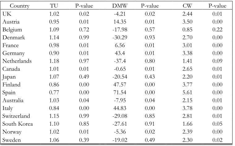
Table 1 shows the results from the estimation of the out-of-sample predictability tests
described in Section 3.1. The null hypothesis in all three tests (TU, DMW and CW) is that
both the consumption-based model and a random walk have the same Mean Squared
Forecast Error (MSFE); the alternative hypothesis is that the model has lower MSFE than a
random walk. We compute all p-values in Table 1 with the bootstrap procedure described in
Section 3.2 and using Equation (30) along with 1000 resamplings to construct the
consumption series and to re-estimate all the predictability tests. This bootstrap procedure is
necessary for the TU and DMW tests to improve their statistical power. The reason for this
feature is that the null hypothesis is nested in the alternative one, see Clark and West (2006,
2007).
Results from the TU and DMW tests are similar to each other for most countries in Table 1.
There is out-of-sample predictability evidence in 10 out of 17 countries according to these
two tests. Countries with no predictability evidence with these tests are Belgium, Denmark,
Netherlands, Japan, Switzerland, South Korea and Sweden.
TABLE 1
Out-of-Sample Exchange Rate Predictability Tests Based on One-Quarter Ahead Forecasts
Country TU P-value DMW P-value CW P-value
UK 1.02 0.02 -4.21 0.02 2.44 0.01
Austria 0.95 0.01 14.35 0.01 3.50 0.00
Belgium 1.09 0.72 -17.98 0.57 0.85 0.22
Denmark 1.14 0.99 -30.29 0.93 2.70 0.00
France 0.98 0.01 6.56 0.01 3.01 0.00
Germany 0.90 0.01 43.4 0.01 3.38 0.00
Netherlands 1.18 0.97 -37.4 0.80 1.41 0.09
Canada 1.01 0.01 -0.65 0.01 2.65 0.01
Japan 1.07 0.49 -20.54 0.43 2.20 0.01
Finland 0.86 0.00 47.57 0.00 3.77 0.00
Spain 0.77 0.00 71.54 0.00 5.61 0.00
Australia 1.03 0.04 -7.95 0.04 2.15 0.01
Italy 0.84 0.00 44.83 0.00 3.78 0.00
Switzerland 1.15 0.99 -29.08 0.85 2.81 0.01
South Korea 1.10 0.85 -27.61 0.91 1.66 0.05
Norway 1.02 0.01 -5.36 0.02 2.39 0.00
Sweden 1.06 0.39 -19.02 0.49 2.30 0.02
This predictability evidence improves when we consider the CW test except in the case of
Belgium. If we only accept null-hypothesis rejections with at least 95% confidence degree,
the CW test reports predictability evidence in 14 out of 17 countries. In this case, there is no
such evidence in Belgium, Netherlands and South Korea.
The reason for the TU and DMW tests to be more stringent than the CW test is that they
directly compare the models in terms of mean square forecasting error (MSFE). In contrast,
the CW test includes the possibility of using a weighted average between the predictions
from the structural and the random-walk models to minimize forecasting errors. In terms of
our results, this finding implies that in the case of Japan, Switzerland and Sweden, we should
combine the consumption-based with the reference model to improve their real exchange
rate forecasts.
This table presents country-by-country out-of-sample predictability tests estimated from Equation (19) using 40-observation rolling samples. We describe the tests TU, DMW and CW in equations (25), (26) and (28) respectively. We compute p-values with the bootstrap
procedure described in Section 3.
In summary, we have found evidence that the consumption-based framework is able to beat
a random walk when forecasting real exchange rates variations one quarter ahead, in 14 out
of 17 economies, using a 95% confidence degree. We show figures of predicted versus
observed real exchange rate variations in the Appendix.
Engel et al (2007) perform similar tests based on panel data regressions, for the same set of
17 countries, using the monetary model of the exchange rate. Although their long-horizon
predictability results are positive for most countries, their short-horizon results work well
only in 4 countries. The failure of the monetary model in predicting exchange rate variations
on short-run horizons relates to its central assumptions. Namely, Purchasing Power Parity
(PPP) and Uncovered Interest Parity (UIP) fail to hold in the short run according to the
literature on international finance10. An alternative explanation for this result is that these
fundamentals have a unit root that, with a near-one discount factor, leads to exchange rates
behaving almost like a random walk, (Engel and West, 2005).
The consumption-based model presented in Section 2 contains an arbitrage condition for
international asset markets and its relation with consumers’ stochastic discount factors
(Equation 11). Therefore, this approach does not need to assume PPP nor UIP in order to
derive the forecasting equation. Additionally, since we use domestic and international
consumption growth as fundamentals, we do not deal with I(1) fundamentals. Finally,
exchange rate predictability in this framework is an implication of the presence of
consumption habits. Namely, it originates on the effects of past consumption growth on
current marginal utility and thus on the expected stochastic discount factors that domestic
and foreign investors use to price international financial assets.
5. ALTERNATIVE FORECASTING WINDOWS
Rogoff and Stavrakeva (2008) argue that it is very important to check for robustness to
alternative rolling-window sizes to assure that the estimated relationship remains stable.11
They perform this kind of robustness check to the exchange rate predictability results from
the models proposed by Molodtsova and Papell (2009), Engel et al (2007) and Gourinchas
and Rey (2007). These exercises show that the out-of-sample predictability evidence weakens
when tests use narrower forecast windows or, equivalently, longer samples to compute the
parameters of the model. The only exception is the international valuation model
(Gourinchas and Rey, 2007) in which the predictability evidence is reasonably stable across
rolling-window sizes.
We perform a similar procedure to evaluate robustness to alternative sizes of the forecasting
window. We focus on the Clark-West test and compute it for each country and for six
alternative sizes that range from 60 to 110 observations, or equivalently, from 80 to 30
observations to compute the regression parameters.
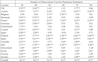
Our results are similar to those in Rogoff and Stavrakeva (2008) for their monetary and
Taylor-rule models. Table 2 shows that the good predictability results from the
consumption-based model remain true when we use 30 to 50 observations to estimate the
parameters of Equation (19). When 60 or 80 observations are employed, this evidence
weakens notoriously across countries. However, when we perform the estimations with a
sample size of 70, there is again predictability evidence for more than a half of the country
sample. These results show the possible time-varying nature of the parameters on the
consumption-based model, especially, those related to external and internal consumption
habits.
TABLE 2
CW Test for Alternative Rolling Forecasting Windows
Number of Observations Used for Parameter Estimation
Country 30 40 50 60 70 80
UK 2.35*** 2.44*** 1.41* 1.15 1.77** 0.86
Austria 1.96** 3.5*** 2.14** 1.52* 2.43*** 2.52***
Belgium -0.90 0.85 1.71** 2.56*** -5.50 NA
Denmark 3.95*** 2.70*** 1.42* 0.95 -0.96 -0.90
France 3.04*** 3.01*** 2.11** 2.10** 2.23** 2.53***
Germany 3.54*** 3.38*** 2.06** 0.53 NA NA
Netherlands 1.75** 1.41* 1.04 2.48 -0.22 NA
Canada 3.18*** 2.65*** 0.79 0.21 1.67** 1.48*
Japan 4.28*** 2.20** 0.99 -0.64 1.34* 0.71
Finland 4.01*** 3.77*** 2.90*** 3.34*** 2.56*** 2.68***
Spain 5.16*** 5.61*** 4.24*** 3.39*** 2.93*** 2.62***
Australia 2.53*** 2.15** 0.79 1.64* 1.80** 0.64
Italy 2.17** 3.78*** 2.45*** 2.52*** 2.59*** 2.28**
Switzerland 1.60* 2.81*** 1.75** 0.69 -1.12 -1.28
Korea 2.08** 1.66** 1.98** 1.84** 1.60* 1.61*
Norway 3.42*** 2.39*** 1.00 0.95 1.39* 1.28
Sweden 2.73*** 2.30** 1.21 1.02 1.88** 1.83**
Overall 16/17 16/17 11/17 8/17 12/17 8/17
6. IN-SAMPLE ESTIMATION OF THE PARAMETERS OF THE MODEL
The goal of this section is to perform a direct, country-by-country estimation of the
structural parameters related to habits, namely: 𝛾𝑖, 𝛾𝑢𝑠 in Equations 20 to 23. We perform
this estimation with a non-linear GMM approach following Hansen (1982). We assume the
remaining parameters to take values according to our data and related literature. Namely, the
average annual consumption growth rate across economies in our dataset of 17 economies
since 1973 is 𝑔 = 2.11%, and its average standard deviation is 𝜎 = 1.51%. We assume an
equal weight for each type of consumption habit, therefore 𝐷 = 0.5. Following the equity
* denotes significance at 10% level; ** denotes significance at 5% level; *** denotes significance at 1% level. NA: not available due to short time series.
This table presents the Clark-West (2006) predictability test for alternative forecasting windows. We evaluate the significance of these tests according to the following asymptotic critical values: 1.282 (10%), 1.645 (5%), 2.33 (1%).
premium literature with habits, for instance Abel (1990), standard values for the time
discount factor and the risk aversion parameter are 𝛽 = 0.95 and 𝛼 = 2, respectively.
The econometric method consists of estimating the sample equivalent of the
conditional expectation of Equation (19) by using country-by-country data on real exchange
rates and consumption growth. Since Equation (19) includes lagged consumption, it is
possible to use contemporaneous consumption-growth measures (domestic, US and world)
as instruments for the GMM estimation. By assumption, the errors from the forecasting
equation remain orthogonal to contemporaneous consumption innovations. As a result, this
set-up gives 4 moment conditions for each country, which allows estimating three
parameters.
We apply the continuously updating GMM estimation method in which the initial
weighting matrix is proportional to 𝑍, the matrix of instruments. Namely, the initial matrix is:
𝑊0 = (𝑍′𝑍)−1. In the second step, we apply the optimal weighting matrix, which is the
inverse of the spectral density matrix. Then we re-estimate this optimal matrix in the
following iterations until an appropriate convergence criterion is reached. Finally, we
compute standard errors following Hansen’s (1982) GMM asymptotic theory12.
Our results show that the habit persistence parameter for each country (𝛾𝑖) is
significantly different from zero in 15 out of 17 countries. The average value of this
parameter, across all the significant cases, is 2.8. Table 3 also shows a country-by-country
estimation of 𝛾𝑢𝑠 which is significant in 11 out of 17 countries and its average value across
countries is 2.0. Therefore, this estimation helps to understand our predictability results by
showing that the presence of habits in the utility function is consistent with the data for most
economies. Thus, open-economy models should analyze in more detail the presence of
consumption habits.
Table 3 also shows the J-test for over-identifying restrictions. This is a test of the null
hypothesis that the estimated parameters are useful to satisfy the moment conditions. The
test detects nine cases, with a 95% confidence degree, for which the selection of instruments
may not be the most appropriate. We regard this result as an implication of fitting a
non-linear equation with only two free parameters. However, if we exclude the cases in which the
J-test detects misspecification with a 95% confidence degree, we still have significant habit
parameters for 7 economies with an average (𝛾𝑖) of 2.4.
TABLE 3
In Sample Non-Linear GMM Estimation of Parameters
Country A. Gamma i B. Gamma US J-Test
UK 5.43* 5.79** 5.07*
Austria 0.35 0.96** 8.89**
Belgium 3.29*** 1.26*** 2.02
Denmark 3.42*** 4.75*** 3.47
France 3.26*** 1.14*** 9.03**
Germany 2.87*** 3.99*** 7.41**
Netherlands 3.27*** 0.82 6.04**
Canada 1.03*** 0.96*** 1.91
Japan 0.67 -0.13 1.36
Finland 3.55*** 1.01*** 8.82**
Spain 3.22*** 0.76* 9.78***
Australia 1.10*** 0.63 3.72
Italy 3.67*** 1.01*** 6.07**
Switzerland 1.24*** 0.45 3.32
Korea 4.68*** 0.02 7.08**
Norway 1.03*** 0.75* 7.76**
Sweden 1.10*** 0.51 5.36*
* denotes significance at 10% level; ** denotes significance at 5% level; *** denotes significance at 1% level.
This table presents country-by-country estimations of habit-related parameters from Equation (19) using the total sample. The method of estimation is non-linear GMM with instrumental variables. The J-test corresponds to the test for over-identifying restrictions.
[image:21.612.182.431.214.448.2]7.
CONCLUSIONS
Engel et al (2007), Rogoff and Stavrakeva (2008), Rossi (2013), among others, explain that it
is difficult to obtain good out-of-sample predictability evidence for the exchange rate in
short-run horizons with the traditional models in the literature. Therefore, the puzzle
described by Meese and Rogoff (1983) still seems to hold in such cases. A few new
approaches have found positive predictability evidence in short-run horizons. Molodtsova
and Papell (2009), Byrne et al (2016) and Ince et al (2016), among others, apply the
Taylor-rule approach. Gourinchas and Rey (2007) employ an external-balance model. Finally, Sarno
and Valente (2009) as well as Fratzscher et al (2015) study scapegoat models of the exchange
rate.
This paper provides an alternative approach to study short-run real exchange rate (RER)
predictability using out-of-sample tests. This framework is an open-economy extension of
the model studied by Abel (1990, 2008), and can be described as a consumption-based
asset-pricing model with N countries and complete markets. In this model, the difference between
Stochastic Discount Factors (SDF) across countries determines real exchange rate variations.
We show that when preferences include internal and external habit persistence, SDFs are
driven by past consumption growth and therefore RER variations are predictable with
consumption data. In other words, habits imply that current consumption growth predict
some of the valuation of financial assets through the effects of current marginal utility on
future SDFs. Furthermore, the functional form of the utility function allows deriving a linear
specification for the RER as function of the following predictors: domestic consumption
growth, US consumption growth and world consumption growth.
Predictability tests with data for 17 developed economies, show good out-of-sample
evidence in 15 countries. Additionally, we confirm the relevance of this habit-based
approach through a direct estimation of the key parameters of the utility function using
non-linear GMM methods. The estimated habit-related parameters are statistically significant for
This consumption-based framework has potential applications for the continuing study of
exchange rate determination. This kind of habit-based utility functions can also be
incorporated to asset pricing models with disaster risk (i.e. Gourio et al, 2013) or long-run
risk (i.e. Colacito and Croce, 2011), in order to develop further results on macro-financial
REFERENCES
Abel, A. (1990). “Asset Prices under Habit Formation and Catching Up with the
Joneses,” American Economic Review, 80(2): 38-42.
Abel, A. (2008). “Equity Premia with Benchmark Levels of Consumption: Closed-Form
Results,” In: Mehra, R. (ed.) Handbook of the Equity Risk Premium: Elsevier, North-Holland, Amsterdam and Boston.
Backus, D., S. Foresi, and C. Telmer, (2001). “Affine Term-Structure Models and the
Forward Premium Anomaly,” Journal of Finance, 56(1): 279-304.
Beckmann, J., and R. Czudaj, (2017). “The Impact of Uncertainty on Professional
Exchange Rate Forecasts,”Journal of International Money and Finance, 73: 296-316.
Campbell, J. and J. Cochrane, (1999). “By Force of Habit: A Consumption-Based
Explanation of Aggregate Stock Market Behavior,” Journal of Political Economy, 107(2): 205–251.
Byrne, J., D. Korobilis, and P. Ribeiro, (2016). “Exchange Rate Predictability in a
Changing World,”Journal of International Money and Finance, 62: 1-24.
Cerra, V., and S. C. Saxena, (2010). “The Monetary Model Strikes Back: Evidence from
the World,”Journal of International Economics, 81(2), 2010, 184-196.
Clark, T. and K. West, (2006). “Using Out-of-Sample Mean Square Prediction Errors to
Test the Martingale Difference Hypothesis,” Journal of Econometrics, 135: 155-186.
Clark, T. and K. West, (2007). “Approximately Normal Tests for Equal Predictive
Accuracy in Nested Models,” Journal of Econometrics, 138(1): 291-311.
Cliff, M, (2003). “GMM and MINZ Program Libraries for MATLAB,” Manuscript.
Cochrane, J, (2005). “Asset Pricing,” Princeton University Press, Princeton NJ, Revised
Edition.
Colacito, R. and M. Croce, (2011). “Risks for the Long Run and the Real Exchange
Rate,” Journal of Political Economy, 119(1): 153-181.
Engel, C., N. Mark and K. West, (2007). “Exchange Rate Models Are Not as Bad as You
Think,” NBER Macroeconomics Annual 2007. Edited by D. Acemoglu, K. Rogoff, and M.
Woodford. National Bureau of Economic Research, Cambridge, MA.
Engel, C., and K. West, (2005). “Exchange Rates and Fundamentals,” The Journal of
Political Economy, 113(3): 485-517.
Fama, E, (1984). “Forward and Spot Exchange Rates,” Journal of Monetary Economics, 14:
319–338.
Foroni, C., F. Ravazzolo, and B. Sadaba, (2018). “Assessing the Predictive Ability of
Sovereign Default Risk on Exchange Rate Returns,” Journal of International Money and
Finance, 81: 242-264.
Fratzscher, M., D. Rime, L. Sarno, and G. Zinna, (2015). “The Scapegoat Theory of
Exchange Rates: The First Tests,”Journal of Monetary Economics, 70: 1-21.
Gourinchas, P. and H. Rey, (2007). “International Financial Adjustment,” Journal of
Political Economy, 115(4): 665-703.
Gourio, F., M. Siemer, and A. Verdelhan, (2013). “International Risk Cycles,” Journal of
International Economics, 89: 471-484.
Groen, J., (2005). “Exchange Rate Predictability and Monetary Fundamentals in a Small
Country Panel,” Journal of Money, Credit and Banking, 37(3): 495-516.
Hansen, L., (1982). “Large Sample Properties of Generalized Method of Moments
Ince, O., T. Molodtsova, and D. Papell, (2016). “Taylor Rule Deviations and
Out-of-Sample Exchange Rate Predictability,”Journal of International Money and Finance, 69: 22-44.
Lustig, H., and A. Verdelhan, (2007). “The Cross-Section of Foreign Currency Risk
Premia and Consumption Growth Risk,” American Economic Review, 97(1): 89-117.
Mark, N., (1995). “Exchange Rates and Fundamentals: Evidence on Long-Horizon
Predictability,” The American Economic Review, 85(1): 201-218.
Mark, N. and D. Sul, (2001). “Nominal Exchange Rates and Monetary Fundamentals:
Evidence from a Small Post Bretton-Woods Panel,” Journal of International Economics, 53:
29-52.
Meese, R. and K. Rogoff, (1983). “Empirical Exchange Rate Models of the Seventies:
Do They Fit Out of Sample?” Journal of International Economics, 14: 3-24.
Molodtsova, T. and D. Papell, (2009). “Out-of-Sample Exchange Rate Predictability with
Taylor Rule fundamentals,” Journal of International Economics, 77: 167-180.
Ojeda-Joya, J. (2014). “A Consumption-Based Approach to Exchange Rate
Predictability,” Borradores de Economia #857, Banco de la Republica, Colombia.
Rogoff, K., (1996). “The Purchasing Power Parity Puzzle,” Journal of Economic Literature,
34(2): 647-668.
Rogoff, K. and V. Stavrakeva, (2008). “The Continuing Puzzle of Short Horizon
Exchange Rate Forecasting,” NBER Working Papers #14701, National Bureau of Economic Research, Cambridge, MA.
Rossi, B. (2013). “Exchange Rate Predictability,” Journal of Economic Literature, 51(4): 1063–1119.
Sarno, L. and G. Valente, (2009). “Exchange Rates and Fundamentals: Footloose or
Taylor, A. and M. Taylor, (2004). “The Purchasing Power Parity Debate,” Journal of
Economic Perspectives, 18(4): 135-158.
Verdelhan, A. (2010). “A Habit-Based Explanation of the Exchange-Rate -risk
Appendix
Figures for Annual Variations of the Real Exchange Rate: Observed
TABLE A1
Weights Used for the Computation of World Consumption
Country GDP 2007 Weight %
Billions of US Dollars
UK 2148 6.6%
Austria 289 0.9%
Belgium 336 1.0%
Denmark 182 0.6%
France 2059 6.3%
Germany 2623 8.0%
Netherlands 567 1.7%
Canada 1127 3.5%
Japan 4229 12.9%
Finland 185 0.6%
Spain 1221 3.7%
Australia 699 2.1%
Italy 1789 5.5%
Switzerland 305 0.9%
Korea 1152 3.5%
Norway 203 0.6%
Sweden 317 1.0%
US 13233 40.5%
Overall 32664 100.0%
This table describes the weights used to compute world consumption in Equation (3). These weights correspond to the relative size of each country's GDP according to the World Development Indicators. The World Bank adjusts these GDP data by purchasing power parity.