1
Deep Generalized Canonical Correlation Analysis
Adrian Benton‡∗ Huda Khayrallah Biman Gujral† Dee Ann Reisinger Sheng Zhang and Raman Arora
‡Bloomberg LP Johns Hopkins University
Abstract
We present Deep Generalized Canonical Cor-relation Analysis (DGCCA) – a method for learning nonlinear transformations of arbitrar-ily many views of data, such that the resulting transformations are maximally informative of each other. While methods for nonlinear
two-view representation learning (Deep CCA, (
An-drew et al.,2013)) and linear many-view
rep-resentation learning (Generalized CCA (Horst,
1961)) exist, DGCCA combines the
flexibil-ity of nonlinear (deep) representation learning with the statistical power of incorporating in-formation from many sources, or views. We present the DGCCA formulation as well as an efficient stochastic optimization algorithm for solving it. We learn and evaluate DGCCA rep-resentations for three downstream tasks: pho-netic transcription from acoustic & articula-tory measurements, recommending hashtags, and recommending friends on a dataset of Twitter users.
1 Introduction
Multiview representation learning refers to set-tings where one has access to many “views” of data at train time. Views often correspond to dif-ferent modalities about examples: a scene repre-sented as a series of audio and image frames, a so-cial media user characterized by the messages they post and who they friend, or a speech utterance and the configuration of the speaker’s tongue. Multi-view techniques learn a representation of data that captures the sources of variation common to all views.
Multiview representation techniques are attrac-tive since a representation that is able to explain many views of the data is more likely to capture meaningful variation than a representation that
∗
Work done while at Johns Hopkins University. †
Now at Google.
is a good fit for only one of the views. These methods are often based on canonical correlation analysis (CCA), a classical statistical technique proposed by Hotelling(1936). CCA-based tech-niques cannot currently model nonlinear relation-ships between arbitrarily many views. Either they are able to model variation across many views, but can only learn linear mappings to the shared space (Horst, 1961), or they can learn nonlinear map-pings, but they cannot be applied to data with more than two views using existing techniques based on Kernel CCA (Hardoon et al.,2004) and Deep CCA (Andrew et al.,2013).
We present Deep Generalized Canonical
Cor-relation Analysis (DGCCA). DGCCA learns a
shared representation from data with arbitrarily many views and simultaneously learns nonlinear mappings from each view to this shared space.Our main methodological contribution is the deriva-tion of the gradient update for the Generalized Canonical Correlation Analysis (GCCA) objective (Horst,1961).1 We evaluate DGCCA-learned rep-resentations on three downstream tasks: (1) pho-netic transcription from aligned speech & articu-latory data, (2) Twitter hashtag and (3) friend rec-ommendation from six text and network feature views. We find that features learned by DGCCA outperform linear multiview techniques on these tasks.
2 Prior Work
Some of the most successful techniques for multi-view representation learning are based on canon-ical correlation analysis and its extension to the nonlinear and many view settings (Wang et al., 2015b,a).
1See https://bitbucket.org/adrianbenton/
Canonical correlation analysis (CCA) Canon-ical correlation analysis (CCA) (Hotelling,1936) is a statistical method that finds maximally cor-related linear projections of two random vectors. It is a fundamental multiview learning technique.
Given two input views, X1 ∈ Rd1 andX2 ∈
Rd2, with covariance matrices, Σ11andΣ22, re-spectively, and cross-covariance matrixΣ12, CCA finds directions that maximize the correlation be-tween these two views:
(u∗1, u∗2) = argmax
u1∈Rd1,u2∈
Rd2
corr(u>1X1, u>2X2)
Since this formulation is invariant to affine trans-formations of u1 and u2, we can write it as the following constrained optimization formulation:
(u∗1, u∗2) = argmax
u1∈Rd1,u2∈Rd2
u>1Σ12u2 (1)
such thatu>1Σ11u1=u>2Σ22u2 = 1. This tech-nique has two limitations that have led to signifi-cant extensions: (1) it is limited to learning rep-resentations that arelineartransformations of the data in each view, and (2) it can only leverage two input views.
Deep Canonical Correlation Analysis (DCCA)
Deep CCA (DCCA) (Andrew et al., 2013)
ad-dresses the first limitation by finding maximally correlatednon-lineartransformations of two vec-tors. It passes each of the input views through neu-ral networks and performs CCA on the outputs.
Let us use f1(X1) = Z1 and f2(X2) = Z2 to represent the network outputs. The weights,
W1andW2, of these networks are trained through standard backpropagation to maximize the CCA objective:
(u∗1, u∗2, W1∗,W2∗) = argmax
u1,u2
corr(u>1Z1, u>2Z2)
Generalized Canonical Correlation Analysis (GCCA) Generalized CCA (GCCA) (Horst, 1961) addresses the limitation on the number of views. It solves the optimization problem in Equa-tion 2, finding a shared representation G of J
different views, where N is the number of data points, dj is the dimensionality of the jth view,
r is the dimensionality of the learned representa-tion, andXj ∈ Rdj×N is the data matrix for the
jth view.
minimize
Uj∈Rdj×r,G∈Rr×N
J
X
j=1
kG−Uj>Xjk2F
subject to GG>=Ir
(2)
Solving GCCA requires finding an eigendecompo-sition of anN ×N matrix, which scales quadrat-ically with sample size and leads to memory con-straints.
Unlike CCA and DCCA, which only learn pro-jections or transformations on each of the views, GCCA also learns a view-independent represen-tation G that best reconstructs all of the view-specific representations simultaneously. The key limitation of GCCA is that it can only learnlinear
transformations of each view.
3 Deep Generalized Canonical Correlation Analysis (DGCCA)
We present Deep GCCA (DGCCA): a multi-view representation learning technique that bene-fits from the expressive power of deep neural net-works and can leverage statistical strength from more than two views. More fundamentally, Deep CCA and Deep GCCA have very different objec-tives and optimization problems, and it is not im-mediately clear how to extend deep CCA to more than two views.
DGCCA learns a nonlinear map for each view in order to maximize the correlation between the learned representations across views. In train-ing, DGCCA passes the input vectors in each view through multiple layers of nonlinear trans-formations and backpropagates the gradient of the GCCA objective with respect to network param-eters to tune each view’s network. The objective is to train networks that reduce the GCCA recon-struction error among their outputs. New data can be projected by feeding each view through its re-spective network.
Problem Consider a dataset of J views and let
Xj ∈Rdj×N denote thejthinput matrix.The
net-work for thejth view consists ofKj layers.
As-sume, for simplicity, that each layer in thejthview network hascj units with a final (output) layer of
size oj. The output of thekth layer for thejth
view ishjk = s(Wkjhjk−1), wheres:R → Ris a
nonlinear activation function andWkj ∈Rck×ck−1
is the weight matrix for the kth layer of the jth
view network. We denote the output of the final layer asfj(Xj).
DGCCA can be expressed as the following op-timization problem: find weight matrices Wj = {W1j, . . . , WKjj } defining the functions fj, and
network), forj= 1, . . . , J, that
minimize
Uj∈Roj×r,G∈Rr×N J
X
j=1
kG−Uj>fj(Xj)k2F (3)
whereG∈Rr×N is the shared representation we
are interested in learning, subject toGG> =Ir.
Optimization We solve the DGCCA optimiza-tion problem using stochastic gradient descent (SGD) with mini-batches. In particular, we es-timate the gradient of the DGCCA objective in Equation 3 on a mini-batch of samples that is mapped through the network and use backpropa-gation to update the weight matrices, Wj’s. Be-cause DGCCA optimization is a constrained opti-mization problem, it is not immediately clear how to perform projected gradient descent with back-propagation. Instead, we characterize the objec-tive function of the GCCA problem at an optimum and compute its gradient with respect to the in-puts to GCCA (i.e. with respect to the network outputs), which are subsequently backpropagated through the network to updateWjs.
Gradient Derivation The solution to the GCCA problem is given by solving an eigenvalue prob-lem. In particular, defineCjj =f(Xj)f(Xj)>∈
Roj×oj, to be the scaled empirical covariance
matrix of the jth network output, and Pj =
f(Xj)>Cjj−1f(Xj) ∈ RN×N to be the
corre-sponding projection matrix that whitens the data; note thatPj is symmetric and idempotent. We
de-fine M = PJ
j=1Pj. Since each Pj is positive
semi-definite, so isM. One can then check that the rows ofGare the topr (orthonormal) eigen-vectors ofM, andUj = Cjj−1f(Xj)G>. Thus, at
the minimum of the objective, we can rewrite the reconstruction error as follows:
J
X
j=1
kG−Uj>fj(Xj)k2F =rJ−Tr(GM G>)
Minimizing the GCCA objective (with respect to the weights of the neural networks) means max-imizingTr(GM G>), which is the sum of eigen-valuesL=Pr
i=1λi(M). Taking the derivative of
Lwith respect to each output layerfj(Xj)gives:
∂L ∂fj(Xj)
= 2UjG−2UjUj>fj(Xj)
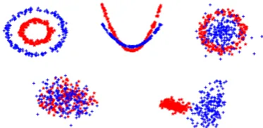
[image:3.595.324.511.64.155.2]Thus, the gradient is the difference between ther -dimensional auxiliary representationGembedded
Figure 1: Three synthetic views are displayed in the top
row, and the bottom rows displays the matrixGlearned
by GCCA (left) and DGCCA (right).
into the subspace spanned by the columns of Uj
(the first term) and the projection of the actual data infj(Xj)onto said subspace (the second term).
4 Experiments
4.1 Synthetic Multiview Mixture Model
We apply DGCCA to a small synthetic data set to show how it preserves the generative structure of data sampled from a multiview mixture model. The three views of the data we use for this experi-ment are plotted in the top row ofFigure 1. Points that share the same color across different views are sampled from the same mixture component.
Importantly, in each view, there is no linear transformation of the data that separates the two
mixture components. This point is reinforced
by Figure 1 (bottom left), which shows the two-dimensional representationGlearned by applying linear GCCA to the data in plotted in the top row. The learned representation completely loses the structure of the data. In contrast, the representa-tionGlearned by DGCCA (bottom right) largely preserves the structure of the data, even after pro-jection onto the first coordinate. In this case, the input neural networks for DGCCA had three hid-den layers with ten units each, with randomly-initialized weights.
4.2 Phoneme Classification
D DH P R B F K SH W AO IY S T HH V UH Y D
DH P R B F K SH W AO IY S T HH V UH
Y 0
10 20 30 40 50 60 70 80 90
D DH P R B F K SH W AO IY S T HH V UH Y D
DH P R B F K SH W AO IY S T HH V UH
Y 0
10 20 30 40 50 60 70 80 90
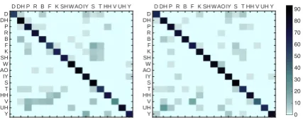
Figure 2: Confusion matrices over phonemes for
speaker-dependent GCCA (left) and DGCCA (right).
K-nearest neighbor classification (Cover and Hart, 1967) is then run on the projected result.
Data We use the same split of the data asArora and Livescu(2014). To limit experiment runtime, we use a subset of speakers for our experiments. We run a set of cross-speaker experiments using the male speaker JW11 for training and two splits of JW24 for tuning and testing. We also perform parameter tuning for the third view with 5-fold cross validation using asingle speaker, JW11. For both experiments, we use acoustic and articulatory measurements as the two views in DCCA. Fol-lowing the pre-processing inAndrew et al.(2013), we get 273 and 112 dimensional feature vectors for the first and second view respectively. Each speaker has∼50,000 frames. For the third view in GCCA and DGCCA, we use 39-dimensional one-hot vectors corresponding to the labels for each frame, followingArora and Livescu(2014).
Parameters We use a fixed network size and regularization for the first two views, each con-taining three hidden layers. Hidden layers for the acoustic view were all width 1024, and lay-ers in the articulatory view all had width 512
units. L2 penalty constants of 0.0001 and
0.01 were placed on the acoustic and articula-tory view networks, with 0.0005 on the label view. The output layer dimension of each net-work is set to 30 for DCCA and DGCCA. For the 5-fold speaker-dependent experiments, we per-formed a grid search for the network sizes in
{128,256,512,1024} and covariance matrix reg-ularization in {10−2,10−4,10−6,10−8} for the third view in each fold. We fix the hyperparame-ters for these experiments optimizing the networks with minibatch stochastic gradient descent with a step size of 0.005, and a batch size of 2,000.
Results DGCCA improves upon both the lin-ear multiview GCCA and the non-linlin-ear 2-view DCCA for both the cross-speaker and
speaker-Table 1: KNN phoneme classification performance.
CROSS-SPEAKER SPEAKER-DEPENDENT
DEV/TEST REC DEV/TEST REC
METHOD ACC ERR ACC ERR
MFCC 48.9/49.3 66.3/66.2
DCCA 45.4/46.1 65.9/65.8
GCCA 49.6/50.2 40.7 69.5/69.8 40.4 DGCCA 53.8/54.2 35.9 72.6/72.3 20.5
dependent cross-validated tasks (Table 1). In addi-tion to accuracy, we examine the reconstrucaddi-tion er-ror (i.e. the objective inEquation 3) obtained from the objective in GCCA and DGCCA. The sharp improvement in reconstruction error shows that a non-linear algorithm can better model the data.
In this experimental setup, DCCA under-performs the baseline of simply running KNN on the original acoustic view. Prior work consid-ered the output of DCCA stacked on to the cen-tral frame of the original acoustic view (39 dimen-sions). This poor performance, in the absence of original features, indicates that it was not able to find a more informative projection than original acoustic features based on correlation with the ar-ticulatory view within the first 30 dimensions.
To highlight the improvements of DGCCA over GCCA,Figure 2presents a subset of the the confu-sion matrices on speaker-dependent test data. We observe large improvements in the classification of
D, F, K, SH,V andY. For instance, DGCCA rectifies the frequent misclassification ofV asP,
R and B by GCCA. In addition, commonly
in-correct classification of phonemes such asS and
T is corrected by DGCCA, which enables better performance on other voiceless consonants such as likeF, KandSH. Vowels are classified with almost equal accuracy by both the methods.
4.3 Hashtag & Friend Recommendation
[image:4.595.72.286.62.147.2]Table 2: Dev/test performance at Twitter friend and hashtag recommendation tasks.
FRIEND HASHTAG
ALGORITHM P@1K R@1K P@1K R@1K
PCA[T+N] .445/.439 .149/.147.011/.008 .312/.290 GCCA[T] .244/.249 .080/.081 .012/.009 .351/.326 GCCA[T+N] .271/.276 .088/.089.012/.010.359/.334 DGCCA[T+N] .297/.268 .099/.090.013/.010 .385/.373
WGCCA[T] .269/.279 .089/.091 .012/.009 .357/.325 WGCCA[T+N] .376/.364 .123/.120 .013/.009 .360/.346
the DGCCA representations on macro precision at 1,000 (P@1K) and recall at 1,000 (R@1K) for the hashtag and friend recommendation tasks de-scribed there.
We trained 40 different DGCCA model
ar-chitectures, each with identical network architec-tures across views, where the width of the hid-den and output layers, c1 and c2, for each view are drawn uniformly from[10,1000], and the aux-iliary representation width r is drawn uniformly from[10, c2].2 All networks used rectified linear units in the hidden layer, and were optimized with Adam (Kingma and Ba, 2014) for 200 epochs. Networks were trained on 90% of 102,328 Twitter users, with 10% of users used as a tuning set to es-timate held-out reconstruction error for model se-lection. We report development and test results for the best performing model on the downstream task development set. The learning rate was set to10−4
with regularization of`1 = 10−2,`2= 10−4.
Table 2 displays the precision and recall at 1000 recommendations of DGCCA compared to PCA[T+N] (PCA applied to concatenation of text and network view feature vectors), linear GCCA applied to the four text views[T], and all text and network views[T+N], along with a GCCA variant with discriminative view weighting (WGCCA). We learned PCA, GCCA, and WGCCA represen-tations of widthr ∈[10,1000], and select embed-dings based on development set R@1K.
There are several points to note: First is that DGCCA outperforms linear methods at hashtag recommendation by a wide margin in terms of recall. This is exciting because this task was shown to benefit from incorporating more than just two views from Twitter users. These results suggest that a nonlinear transformation of the
in-2
We only consider architectures with single-hidden-layer networks identical across views so as to avoid a fishing ex-pedition. If DGCCA is an appropriate method for learning Twitter user embeddings, then it should require little archi-tecture exploration.
put views can yield additional gains in perfor-mance. In addition, WGCCA models sweep over every possible weighting of views with weights in
{0,0.25,1.0}. The fact that DGCCA is able to outperform WGCCA at hashtag recommendation is encouraging, since WGCCA has much more freedom to discard uninformative views. As noted in Benton et al. (2016), only the friend network view was useful for learning representations for friend recommendation (corroborated by perfor-mance of PCA applied to friend network view), so it is unsurprising that DGCCA, when applied to all views, cannot compete with WGCCA representa-tions learned on the single useful friend network view.
5 Discussion
There has also been strong work outside of CCA-related methods to combine nonlinear representa-tion and learning from multiple views. Kumar et al. (2011) outlines two main approaches to learn a joint representation from many views: either by (1) explicitly maximizing similarity/correlation between view pairs (Masci et al., 2014; Rajen-dran et al.,2015) or by (2) alternately optimizing a shared, “consensus” representation and view-specific transformations (Kumar et al., 2011; Xi-aowen, 2014; Sharma et al., 2012). Unlike the first class of methods, the complexity of solving DGCCA does not scale quadratically with num-ber of views, nor does it require a privileged pivot view (G is learned). Unlike methods that esti-mate a “consensus” representation, DGCCA ad-mits a globally optimal solution for both the view-specific projectionsU1. . . UJ, and the shared
rep-resentationG. Local optima arise in the DGCCA objective only because we are also learning non-linear transformations of the input views.
References
Galen Andrew, Raman Arora, Jeff Bilmes, and Karen Livescu. 2013. Deep canonical correlation analysis. InProceedings of the 30th International Conference on Machine Learning, pages 1247–1255.
Raman Arora and Karen Livescu. 2014. Multi-view learning with supervision for transformed bottleneck
features. InAcoustics, Speech and Signal
Process-ing (ICASSP), 2014 IEEE International Conference
on, pages 2499–2503. IEEE.
Adrian Benton, Raman Arora, and Mark Dredze. 2016. Learning multiview embeddings of twitter users. In
The 54th Annual Meeting of the Association for Computational Linguistics, page 14.
Thomas M Cover and Peter E Hart. 1967. Nearest
neighbor pattern classification. Information Theory,
IEEE Transactions on, 13(1):21–27.
David R Hardoon, Sandor Szedmak, and John Shawe-Taylor. 2004. Canonical correlation analysis: An overview with application to learning methods.
Neural computation, 16(12):2639–2664.
Paul Horst. 1961. Generalized canonical correlations
and their applications to experimental data. Journal
of Clinical Psychology, 17(4).
Harold Hotelling. 1936. Relations between two sets of
variates. Biometrika, pages 321–377.
Diederik Kingma and Jimmy Ba. 2014. Adam: A
method for stochastic optimization. arXiv preprint
arXiv:1412.6980.
Abhishek Kumar, Piyush Rai, and Hal Daume. 2011.
Co-regularized multi-view spectral clustering. In
Advances in neural information processing systems, pages 1413–1421.
Jonathan Masci, Michael M Bronstein, Alexander M Bronstein, and J¨urgen Schmidhuber. 2014.
Multi-modal similarity-preserving hashing. IEEE
transac-tions on pattern analysis and machine intelligence, 36(4):824–830.
Janarthanan Rajendran, Mitesh M Khapra, Sarath Chandar, and Balaraman Ravindran. 2015. Bridge correlational neural networks for multilingual
mul-timodal representation learning. arXiv preprint
arXiv:1510.03519.
Abhishek Sharma, Abhishek Kumar, Hal Daume, and David W Jacobs. 2012. Generalized multiview
anal-ysis: A discriminative latent space. InComputer
Vi-sion and Pattern Recognition (CVPR), 2012 IEEE Conference on, pages 2160–2167. IEEE.
Weiran Wang, Raman Arora, Karen Livescu, and Jeff Bilmes. 2015a. On deep multi-view representation
learning. In Proc. of the 32nd Int. Conf. Machine
Learning (ICML 2015).
Weiran Wang, Raman Arora, Karen Livescu, and Jeff Bilmes. 2015b. Unsupervised learning of acoustic features via deep canonical correlation analysis. In
Proc. of the IEEE Int. Conf. Acoustics, Speech and Sig. Proc. (ICASSP’15).
John R. Westbury. 1994. X-ray microbeam speech
pro-duction database user’s handbook. InWaisman
Cen-ter on Mental Retardation & Human Development University of Wisconsin Madison, WI 53705-2280.
Dong Xiaowen. 2014. Multi-View Signal Processing