2462
End-to-End Reinforcement Learning for Automatic Taxonomy Induction
Yuning Mao1, Xiang Ren2, Jiaming Shen1, Xiaotao Gu1, Jiawei Han1
1Department of Computer Science, University of Illinois Urbana-Champaign, IL, USA
2Department of Computer Science, University of Southern California, CA, USA
1{yuningm2, js2, xiaotao2, hanj}@illinois.edu 2[email protected]
Abstract
We present a novel end-to-end reinforce-ment learning approach to automatic tax-onomy induction from a set of terms. While prior methods treat the problem as a two-phase task (i.e., detecting hypernymy pairs followed by organizing these pairs into a tree-structured hierarchy), we ar-gue that such two-phase methods may suf-fer from error propagation, and cannot ef-fectively optimize metrics that capture the holistic structure of a taxonomy. In our ap-proach, the representations of term pairs are learned using multiple sources of in-formation and used to determine which term to select andwhereto place it on the taxonomy via a policy network. All com-ponents are trained in an end-to-end man-ner with cumulative rewards, measured by a holistic tree metric over the train-ing taxonomies. Experiments on two pub-lic datasets of different domains show that our approach outperforms prior state-of-the-art taxonomy induction methods up to 19.6% on ancestor F1.1
1 Introduction
Many tasks in natural language understanding (e.g., information extraction (Demeester et al.,
2016), question answering (Yang et al.,2017), and textual entailment (Sammons,2012)) rely on lexi-cal resources in the form of term taxonomies (cf. rightmost column in Fig.1). However, most exist-ing taxonomies, such as WordNet (Miller, 1995) and Cyc (Lenat,1995), are manually curated and thus may have limited coverage or become un-available in some domains and languages. There-fore, recent efforts have been focusing on auto-matic taxonomy induction, which aims to organize 1Code and data can be found at https://github. com/morningmoni/TaxoRL
a set of terms into a taxonomy based on relevant resources such as text corpora.
Prior studies on automatic taxonomy induc-tion (Gupta et al.,2017;Camacho-Collados,2017) often divide the problem into two sequential sub-tasks: (1) hypernymy detection (i.e., extracting term pairs of “is-a” relation); and (2) hyper-nymy organization(i.e., organizing is-a term pairs into a tree-structured hierarchy). Methods devel-oped for hypernymy detection either harvest new terms (Yamada et al.,2009;Kozareva and Hovy,
2010) or presume a vocabulary is given and study term semantics (Snow et al.,2005;Fu et al.,2014;
Tuan et al.,2016;Shwartz et al.,2016). The hy-pernymy pairs extracted in the first subtask form a noisy hypernym graph, which is then transformed into a tree-structured taxonomy in the hypernymy organization subtask, using different graph prun-ing methods includprun-ing maximum spannprun-ing tree (MST) (Bansal et al., 2014;Zhang et al., 2016), minimum-cost flow (MCF) (Gupta et al., 2017) and other pruning heuristics (Kozareva and Hovy,
2010; Velardi et al., 2013; Faralli et al., 2015;
Panchenko et al.,2016).
proba-affenpinscher miniature_pinscher pinscher
collie shepherd_dog
Appenzeller Sennenhunde
working_dog root
affenpinscher miniature_pinscher pinscher
Appenzeller Sennenhunde
working_dog
miniature_pinscher pinscher
Appenzeller Sennenhunde
working_dog
[image:2.595.73.535.60.122.2]t=0 t=5 t=6 t=8
Figure 1: An illustrative example showing the process of taxonomy induction. The input vocabulary
V0 is{“working dog”, “pinscher”, “shepherd dog”, ...}, and the initial taxonomyT0 is empty. We use a virtual “root” node to representT0 att = 0. At timet = 5, there are 5 terms on the taxonomy T5 and 3 terms left to be attached: Vt = {“shepherd dog”, “collie”, “affenpinscher”}. Suppose the term
“affenpinscher” is selected and put under “pinscher”, then the remaining vocabularyVt+1 at next time step becomes{“shepherd dog”, “collie”}. Finally, after|V0|time steps, all the terms are attached to the taxonomy andV|V0|=V8={}. A full taxonomy is then constructed from scratch.
bilities to represent the taxonomy quality. How-ever, the edges are treated equally, while in reality, they contribute to the taxonomy differently. For example, a high-level edge is likely to be more important than a bottom-out edge because it has much more influence on its descendants. In ad-dition, these methods cannotexplicitlycapture the holistic taxonomy structure by optimizing global metrics.
To address the above issues, we propose to jointly conduct hypernymy detection and organi-zation by learning term pair representations and constructing the taxonomy simultaneously. Since it is infeasible to estimate the quality of all pos-sible taxonomies, we design an end-to-end rein-forcement learning (RL) model to combine the two phases. Specifically, we train an RL agent that employs the term pair representations using multi-ple sources of information and determines which term to select and where to place it on the tax-onomy via a policy network. The feedback from hypernymy organization is propagated back to the hypernymy detection phase, based on which the term pair representations are adjusted. All compo-nents are trained in an end-to-end manner with cu-mulative rewards, measured by a holistic tree met-ric over the training taxonomies. The probability of a full taxonomy is no longer a simple aggre-gated probability of its edges. Instead, we assess an edge based on how much it can contribute to the whole quality of the taxonomy.
We perform two sets of experiments to eval-uate the effectiveness of our proposed approach. First, we test the end-to-end taxonomy induction performance by comparing our approach with the state-of-the-art two-phase methods, and show that our approach outperforms them significantly on
the quality of constructed taxonomies. Second, we use the same (noisy) hypernym graph as the input of all compared methods, and demonstrate that our RL approach does better hypernymy organization through optimizing metrics that can capture holis-tic taxonomy structure.
Contributions. In summary, we have made the
following contributions: (1) We propose a deep reinforcement learning approach to unify hyper-nymy detection and organization so as to induct taxonomies in an end-to-end manner. (2) We de-sign a policy network to incorporate semantic in-formation of term pairs and use cumulative re-wards to measure the quality of constructed tax-onomies holistically. (3) Experiments on two pub-lic datasets from different domains demonstrate the superior performance of our approach com-pared with state-of-the-art methods. We also show that our method can effectively reduce error prop-agation and capture global taxonomy structure.
2 Automatic Taxonomy Induction
2.1 Problem Definition
2.2 Modeling Hypernymy Relation
Determining which term to select from V0 and where to place it on the current hierarchy requires understanding of the semantic relationships be-tween the selected term and all the other terms. We consider multiple sources of information (i.e., resources) for learning hypernymy relation rep-resentations of term pairs, including dependency path-based contextual embedding and distribu-tional term embeddings (Shwartz et al.,2016).
Path-based Information. We extract the shortest
dependency paths between each co-occurring term pair from sentences in the given background cor-pora. Each path is represented as a sequence of edges that goes from term xto term y in the de-pendency tree, and each edge consists of the word lemma, the part-of-speech tag, the dependency la-bel and the edge direction between two contiguous words. The edge is represented by the concatena-tion of embeddings of its four components:
Ve = [Vl, ,Vpos,Vdep,Vdir].
Instead of treating the entire dependency path as a single feature, we encode the sequence of de-pendency edgesVe1,Ve2, ...,Vek using an LSTM so that the model can focus on learning from parts of the path that are more informative while ig-noring others. We denote the final output of the LSTM for pathpasOp, and useP(x, y)to
repre-sent the set of all dependency paths between term pair (x, y). A single vector representation of the term pair (x, y) is then computed as PP(x,y), the weighted average of all its path representations by applying an average pooling:
PP(x,y)=
∑
p∈P(x,y)c(x,y)(p)·Op ∑
p∈P(x,y)c(x,y)(p)
,
wherec(x,y)(p)denotes the frequency of pathpin
P(x, y). For those term pairs without dependency paths, we use a randomly initializedempty pathto represent them as in Shwartz et al.(2016).
Distributional Term Embedding. The previous
path-based features are only applicable when two terms co-occur in a sentence. In our experiments, however, we found that only about 17% of term pairs have sentence-level co-occurrences.2 To al-leviate the sparse co-occurrence issue, we concate-nate the path representationPP(x,y)with the word 2In comparison, more than 70% of term pairs have
sentence-level co-occurrences in BLESS (Baroni and Lenci,
2011), a standard hypernymy detection dataset.
embeddings ofx andy, which capture the distri-butional semantics of two terms.
Surface String Features. In practice, even the
embeddings of many terms are missing because the terms in the input vocabulary may be multi-word phrases, proper nouns or named entities, which are likely not covered by the external pre-trained word embeddings. To address this issue, we utilize several surface features described in previous studies (Yang and Callan, 2009; Bansal et al.,2014;Zhang et al.,2016). Specifically, we employCapitalization,Ends with,Contains,Suffix match,Longest common substringandLength dif-ference. These features are effective for detecting hypernyms solely based on the term pairs.
Frequency and Generality Features. Another
feature source that we employ is the hyper-nym candidates from TAXI3 (Panchenko et al.,
2016). These hypernym candidates are extracted by lexico-syntactic patterns and may be noisy. As only term pairs and the co-occurrence frequen-cies of them (under specific patterns) are available, we cannot recover the dependency paths between these terms. Thus, we design two features that are similar to those used in (Panchenko et al., 2016;
Gupta et al.,2017).4
• Normalized Frequency Diff. For a hyponym-hypernym pair (xi, xj) where xi is the
hy-ponym and xj is the hypernym, its
normal-ized frequency is defined as freqn(xi, xj) =
freq(xi,xj)
maxkfreq(xi,xk), where freq(xi, xj) denotes the
raw frequency of (xi, xj). The final
fea-ture score is defined as freqn(xi, xj) −
freqn(xj, xi), which down-ranks synonyms and
co-hyponyms. Intuitively, a higher score in-dicates a higher probability that the term pair holds the hypernymy relation.
• Generality Diff.The generalityg(x)of a termx
is defined as the logarithm of the number of its distinct hyponyms,i.e.,g(x) =log(1+|hypo|), where for anyhypo∈hypo,(hypo, x)is a hy-pernym candidate. A high g(x) of the term x
implies thatx is general since it has many dis-tinct hyponyms. The generality of a term pair is defined as the difference in generality between
xj andxi: g(xj)−g(xi). This feature would
3
http://tudarmstadt-lt.github.io/taxi/
4Since the features use additional resource, we wouldn’t
promote term pairs with the right level of gener-ality and penalize term pairs that are either too general or too specific.
The surface, frequency, and generality features are binned and their embeddings are concatenated as a part of the term pair representation. In sum-mary, the final term pair representation Rxy has
the following form:
Rxy = [PP(x,y),Vwx,Vwy,VF(x,y)],
wherePP(x,y),Vwx,Vwy,VF(x,y)denote the path representation, the word embedding of x and y, and the feature embeddings, respectively.
Our approach is general and can be flexibly ex-tended to incorporate different feature representa-tion components introduced by other relarepresenta-tion ex-traction models (Zhang et al., 2017; Lin et al.,
2016; Shwartz et al., 2016). We leave in-depth discussion of the design choice of hypernymy re-lation representation components as future work.
3 Reinforcement Learning for End-to-End Taxonomy Induction
We present the reinforcement learning (RL) ap-proach to taxonomy induction in this section. The RL agent employs the term pair representations described in Section 2.2 as input, and explores how to generate a whole taxonomy by selecting one term at each time step and attaching it to the current taxonomy. We first describe the environ-ment, including the actions, states, and rewards. Then, we introduce how to choose actions via a policy network.
3.1 Actions
We regard the process of building a taxonomy as making a sequence of actions. Specifically, we de-fine that an action at at time step t is to (1)
se-lect a termx1 from the remaining vocabularyVt;
(2) removex1 fromVt, and (3) attachx1as a hy-ponym of one termx2 that is already on the cur-rent taxonomy Tt. Therefore, the size of action
space at time step t is |Vt| × |Tt|, where |Vt|is
the size of the remaining vocabulary Vt, and|Tt|
is the number of terms on the current taxonomy. At the beginning of each episode, the remaining vocabularyV0is equal to the input vocabulary and the taxonomyT0 is empty. During the taxonomy induction process, the following relations always hold: |Vt| = |Vt−1| −1, |Tt| = |Tt−1|+ 1, and
|Vt|+|Tt| = |V0|. The episode terminates when all the terms are attached to the taxonomy, which makes the length of one episode equal to|V0|.
A remaining issue is how to select the first term when no terms are on the taxonomy. One approach that we tried is to add a virtual node as root and consider it as if a real node. Theroot embedding is randomly initialized and updated with other pa-rameters. This approach presumes that all tax-onomies share a common root representation and expects to find the real root of a taxonomy via the term pair representations between the virtual root and other terms. Another approach that we ex-plored is to postpone the decision of root by ini-tializingT with a random term as current root at the beginning of one episode, and allowing the se-lection of new rootby attaching one term as the hypernym of current root. In this way, it over-comes the lack of prior knowledge when the first term is chosen. The size of action space then be-comes|At|=|Vt| × |Tt|+|Vt|, and the length of
one episode becomes |V0| −1. We compare the performance of the two approaches in Section4.
3.2 States
Thestatesat timetcomprises the current taxon-omyTtand the remaining vocabularyVt. At each
time step, the environment provides the informa-tion of current state, based on which the RL agent takes an action. Once a term pair(x1, x2) is se-lected, the position of the new termx1is automati-cally determined since the other termx2is already on the taxonomy and we can simply attachx1 by adding an edge betweenx1andx2.
3.3 Rewards
The agent takes a scalar reward as feedback of its actions to learn its policy. One obvious re-ward is to wait until the end of taxonomy induc-tion, and then compare the predicted taxonomy with gold taxonomy. However, this reward is de-layed and difficult to measure individual actions in our scenario. Instead, we use reward shap-ing,i.e., giving intermediate rewards at each time step, to accelerate the learning process. Empir-ically, we set the reward r at time step t to be the difference of Edge-F1 (defined in Section4.2
and evaluated by comparing the current taxonomy with the gold taxonomy) between current and last time step: rt = F1et −F1et−1. If current
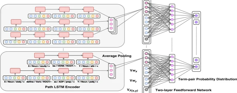
cumula-Figure 2: The architecture of the policy network. The dependency paths are encoded and concatenated with word embeddings and feature embeddings, and then fed into a two-layer feed-forward network.
tive reward from current time step to the end of an episode would cancel the intermediate rewards and thus reflect whether current action improves the overall performance or not. As a result, the agent would not focus on the selection of current term pair but have a long-term view that takes fol-lowing actions into account. For example, suppose there are two actions at the same time step. One action attaches a leaf node to a high-level node, and the other action attaches a non-leaf node to the same high-level node. Both attachments form a wrong edge but the latter one is likely to receive a higher cumulative reward because its following attachments are more likely to be correct.
3.4 Policy Network
After we introduce the term pair representations and define the states, actions, and rewards, the problem becomes how to choose an action from the action space, i.e., which term pair (x1, x2) should be selected given the current state? To solve the problem, we parameterize each actiona
by a policy networkπ(a|s;WRL). The
architec-ture of our policy network is shown in Fig.2. For each term pair, its representation is obtained by the path LSTM encoder, the word embeddings of both terms, and the embeddings of features. By stack-ing the term pair representations, we can obtain an action matrixAtwith size(|Vt| × |Tt|)×dim(R),
where(|Vt| × |Tt|)denotes the number of
possi-ble actions (term pairs) at timetanddim(R) de-notes the dimension of term pair representationR.
At is then fed into a two-layer feed-forward
net-work followed by a softmax layer which outputs
the probability distribution of actions.5Finally, an actionatis sampled based on the probability
dis-tribution of the action space:
Ht=ReLU(W1RLATt +b1RL), π(a|s;WRL) =softmax(W2RLHt+b2RL),
at∼π(a|s;WRL).
At the time of inference, instead of sampling an action from the probability distribution, we greed-ily select the term pair with the highest probability. We useREINFORCE(Williams,1992), one in-stance of the policy gradient methods as the opti-mization algorithm. Specifically, for each episode, the weights of the policy network are updated as follows:
WRL=WRL+α
T ∑
t=1
∇logπ(at|s;WRL)·vt,
wherevi = ∑T
t=iγt−irtis the culmulative future
reward at time i andγ ∈ [0,1] is a discounting factor of future rewards.
To reduce variance, 10 rollouts for each training sample are run and the rewards are averaged. An-other common strategy for variance reduction is to use a baseline and give the agent the difference between the real reward and the baseline reward instead of feeding the real reward directly. We use a moving average of the reward as the baseline for simplicity.
5
[image:5.595.91.503.66.228.2]3.5 Implementation Details
We use pre-trained GloVe word vectors ( Penning-ton et al., 2014) with dimensionality 50 as word embeddings. We limit the maximum number of dependency paths between each term pair to be 200 because some term pairs containing general terms may have too many dependency paths. We run with different random seeds and hyperparam-eters and use the validation set to pick the best model. We use an Adam optimizer with initial learning rate10−3. We set the discounting factorγ
to 0.4 as it is shown that using a smaller discount factor than defined can be viewed as regulariza-tion (Jiang et al.,2015). Since the parameter up-dates are performed at the end of each episode, we cache the term pair representations and reuse them when the same term pairs are encountered again in the same episode. As a result, the proposed ap-proach is very time efficient – each training epoch takes less than 20 minutes on a single-core CPU using DyNet (Neubig et al.,2017).
4 Experiments
We design two experiments to demonstrate the ef-fectiveness of our proposed RL approach for tax-onomy induction. First, we compare our end-to-end approach with two-phase methods and show that our approach yields taxonomies with higher quality through reducing error propagation and optimizing towards holistic metrics. Second, we conduct a controlled experiment on hypernymy organization, where the same hypernym graph is used as the input of both our approach and the compared methods. We show that our RL method is more effective at hypernymy organization.
4.1 Experiment Setup
Here we introduce the details of our two experi-ments on validating that (1) the proposed approach can effectively reduce error propagation; and (2) our approach yields better taxonomies via opti-mizing metrics on holistic taxonomy structure.
Performance Study on End-to-End Taxonomy
Induction. In the first experiment, we show that
our joint learning approach is superior to two-phase methods. Towards this goal, we compare with TAXI (Panchenko et al., 2016), a typical two-phase approach, two-phase HypeNET, im-plemented by pairwise hypernymy detection and hypernymy organization using MST, and Bansal
et al.(2014). The dataset we use in this experi-ment is fromBansal et al.(2014), which is a set of medium-sized full-domain taxonomies consisting of bottom-out full subtrees sampled from Word-Net. Terms in different taxonomies are from var-ious domains such as animals, general concepts, daily necessities. Each taxonomy is of height four (i.e., 4 nodes from root to leaf) and contains (10, 50] nodes. The dataset contains 761 non-overlapped taxonomies in total and is partitioned by 70/15/15% (533/114/114) as training, valida-tion, and test set, respectively.
Testing on Hypernymy Organization. In the
second experiment, we show that our approach is better at hypernymy organization by leverag-ing the global taxonomy structure. For a fair comparison, we reuse the hypernym graph as in TAXI (Panchenko et al.,2016) and SubSeq (Gupta et al.,2017) so that the inputs of each model are the same. Specifically, we restrict the action space to be the same as the baselines by considering only term pairs in the hypernym graph, rather than all
|V|×|T|possible term pairs. As a result, it is pos-sible that at some point no more hypernym candi-dates can be found but the remaining vocabulary is still not empty. If the induction terminates at this point, we call it apartial induction. We can also continue the induction by restoring the original ac-tion space at this moment so that all the terms inV
are eventually attached to the taxonomy. We call this setting a full induction. In this experiment, we use the English environment and science tax-onomies in the SemEval-2016 task 13 (TExEval-2) (Bordea et al., 2016). Each taxonomy is com-posed of hundreds of terms, which is much larger than the WordNet taxonomies. The taxonomies are aggregated from existing resources such as WordNet, Eurovoc6, and the Wikipedia Bitaxon-omy (Flati et al.,2014). Since this dataset provides no training data, we train our model using the WordNet dataset in the first experiment. To avoid possible overlap between these two sources, we exclude those taxonomies constructed from Word-Net.
In both experiments, we combine three pub-lic corpora – the latest Wikipedia dump, the UMBC web-based corpus (Han et al., 2013) and the One Billion Word Language Modeling Bench-mark (Chelba et al.,2013). Only sentences where term pairs co-occur are reserved, which results in
Model Pa Ra F1a Pe Re F1e TAXI 66.1 13.9 23.0 54.8 18.0 27.1 HypeNET 32.8 26.7 29.4 26.1 17.2 20.7 HypeNET+MST 33.7 41.1 37.0 29.2 29.2 29.2 TaxoRL (RE) 35.8 47.4 40.8 35.4 35.4 35.4 TaxoRL (NR) 41.3 49.2 44.9 35.6 35.6 35.6
Bansal et al.(2014) 48.0 55.2 51.4 - -
[image:7.595.309.525.61.171.2]-TaxoRL (NR) + FG 52.9 58.6 55.6 43.8 43.8 43.8
Table 1: Results of the end-to-end taxonomy in-duction experiment. Our approach significantly outperforms two-phase methods (Panchenko et al.,
2016;Shwartz et al., 2016;Bansal et al., 2014).
Bansal et al.(2014) and TaxoRL (NR) + FG are listed separately because they use extra resources.
a corpus with size 2.6 GB for the WordNet dataset and 810 MB for the TExEval-2 dataset. Depen-dency paths between term pairs are extracted from the corpus via spaCy7.
4.2 Evaluation Metrics
Ancestor-F1. It compares the ancestors (“is-a”
pairs) on the predicted taxonomy with those on the gold taxonomy. We usePa,Ra,F1ato denote the
precision, recall, and F1-score, respectively:
Pa= |
is-asys∧is-agold|
|is-asys|
, Ra= |
is-asys∧is-agold|
|is-agold|
.
Edge-F1. It is more strict thanAncestor-F1since
it only compares predicted edges with gold edges. Similarly, we denote edge-based metrics as Pe, Re, andF1e, respectively. Note thatPe = Re = F1eif the number of predicted edges is the same
as gold edges.
4.3 Results
Comparison on End-to-End Taxonomy Induc-tion. Table1 shows the results of the first exper-iment. HypeNET (Shwartz et al.,2016) uses ad-ditional surface features described in Section2.2. HypeNET+MST extends HypeNET by first con-structing a hypernym graph using HypeNET’s out-put as weights of edges and then finding the MST (Chu, 1965) of this graph. TaxoRL (RE) denotes our RL approach which assumes a com-monRoot Embedding, and TaxoRL (NR) denotes its variant that allows aNew Rootto be added.
We can see that TAXI has the lowestF1awhile
HypeNET performs the worst inF1e. Both TAXI
and HypeNET’sF1aandF1e are lower than 30.
HypeNET+MST outperforms HypeNET in both
7https://spacy.io/
Model Pa Ra F1a Pe Re F1e
Env
TAXI (DAG) 50.1 32.7 39.6 33.8 26.8 29.9 TAXI (tree) 67.5 30.8 42.3 41.1 23.1 29.6
SubSeq - - - 22.4
TaxoRL (Partial) 51.6 36.4 42.7 37.5 24.2 29.4 TaxoRL (Full) 47.2 54.6 50.6 32.3 32.3 32.3
Sci
TAXI (DAG) 61.6 41.7 49.7 38.8 34.8 36.7 TAXI (tree) 76.8 38.3 51.1 44.8 28.8 35.1
SubSeq - - - 39.9
TaxoRL (Partial) 84.6 34.4 48.9 56.9 33.0 41.8 TaxoRL (Full) 68.3 52.9 59.6 37.9 37.9 37.9
Table 2: Results of the hypernymy orga-nization experiment. Our approach outper-formsPanchenko et al.(2016);Gupta et al.(2017) when the same hypernym graph is used as input. The precision of partial induction in both metrics is high. The precision of full induction is relatively lower but its recall is much higher.
F1aandF1e, because it considers the global
tax-onomy structure, although the two phases are per-formed independently. TaxoRL (RE) uses ex-actly the same input as HypeNET+MST and yet achieves significantly better performance, which demonstrates the superiority of combining the phases of hypernymy detection and hypernymy organization. Also, we found that presuming a shared root embedding for all taxonomies can be inappropriate if they are from different domains, which explains why TaxoRL (NR) performs bet-ter than TaxoRL (RE). Finally, afbet-ter we add the frequency and generality features (TaxoRL (NR) + FG), our approach outperforms Bansal et al.
(2014), even if a much smaller corpus is used.8
Analysis on Hypernymy Organization. Table2
lists the results of the second experiment. TAXI (DAG) (Panchenko et al., 2016) denotes TAXI’s original performance on the TExEval-2 dataset.9 Since we don’t allow DAG in our setting, we con-vert its results to trees (denoted by TAXI (tree)) by only keeping the first parent of each node. Sub-Seq (Gupta et al., 2017) also reuses TAXI’s hy-pernym candidates. TaxoRL (Partial) and Tax-oRL (Full) denotes partial induction and full in-duction, respectively. Our joint RL approach out-performs baselines in both domains substantially. TaxoRL (Partial) achieves higher precision in both ancestor-based and edge-based metrics but has
rel-8Bansal et al.(2014) use an unavailable resource (Brants
and Franz,2006) which contains one trillion tokens while our
public corpus contains several billion tokens. The frequency and generality features are sparse because the vocabulary that TAXI (in the TExEval-2 competition) used for focused crawl-ing and hypernymy detection was different.
atively lower recall since it discards some terms. In addition, it achieves the best F1e in science
domain. TaxoRL (Full) has the highest recall in both domains and metrics, with the compromise of lower precision. Overall, TaxoRL (Full) per-forms the best in both domains in terms of F1a
and achieves bestF1ein environment domain.
5 Ablation Analysis and Case Study
In this section, we conduct ablation analysis and present a concrete case for better interpreting our model and experimental results.
Table 3 shows the ablation study of TaxoRL (NR) on the WordNet dataset. As one may find, different types of features are complementary to each other. Combining distributional and path-based features performs better than using either of them alone (Shwartz et al.,2016). Adding surface features helps model string-level statistics that are hard to capture by distributional or path-based fea-tures. Significant improvement is observed when more data is used, meaning that standard corpora (such as Wikipedia) might not be enough for com-plicated taxonomies like WordNet.
Fig.3shows the results of taxonomy about fil-ter. We denote the selected term pair at time step
tas (hypo, hyper,t). Initially, the termwater filter is randomly chosen as the taxonomy root. Then, a wrong term pair (water filter, air filter, 1) is se-lected possibly due to the noise and sparsity of fea-tures, which makes the termair filterbecome the new root. (air filter, filter, 2) is selected next and the current root becomesfilterthat is identical to the real root. After that, term pairs such as (fuel filter, filter, 3), (coffee filter, filter, 4) are selected correctly, mainly because of the substring inclu-sion intuition. Other term pairs such as (colander, strainer, 13), (glass wool, filter, 16) are discovered later, largely by the information encoded in the de-pendency paths and embeddings. For those undis-covered relations, (filter tip, air filter) has no de-pendency path in the corpus. sifteris attached to the taxonomy before its hypernymsieve. There is no co-occurrence betweenbacteria bed (ordrain basket) and other terms. In addition, it is hard to utilize the surface features since they “look differ-ent” from other terms. That is also why (bacteria bed, air filter, 17) and (drain basket, air filter, 18) are attached in the end: our approach prefers to select term pairs with high confidence first.
Model Pa Ra F1a F1e
Distributional Info 27.1 24.3 25.6 13.8 Path-based Info 27.8 48.5 33.7 27.4 D+P 36.6 39.4 37.9 28.3 D+P+Surface Features 41.3 49.2 44.9 35.6 D+P+S+ FG 52.9 58.6 55.6 43.8
Table 3: Ablation study on the WordNet dataset (Bansal et al.,2014). Pe andReare
omit-ted because they are the same as F1e for each
model. We can see that our approach benefits from multiple sources of information which are comple-mentary to each other.
6 Related Work
6.1 Hypernymy Detection
Finding high-quality hypernyms is of great impor-tance since it serves as the first step of taxonomy induction. In previous works, there are mainly two categories of approaches for hypernymy de-tection, namely pattern-based and distributional methods. Pattern-based methods consider lexico-syntactic patterns between the joint occurrences of term pairs for hypernymy detection. They gen-erally achieve high precision but suffer from low recall. Typical methods that leverage patterns for hypernym extraction include (Hearst,1992;Snow et al.,2005;Kozareva and Hovy,2010;Panchenko et al.,2016;Nakashole et al.,2012). Distributional methods leverage the contexts of each term sepa-rately. The co-occurrence of term pairs is hence unnecessary. Some distributional methods are de-veloped in an unsupervised manner. Measures such as symmetric similarity (Lin et al.,1998) and those based on distributional inclusion hypothe-sis (Weeds et al.,2004;Chang et al.,2017) were proposed. Supervised methods, on the other hand, usually have better performance than unsuper-vised methods for hypernymy detection. Recent works towards this direction include (Fu et al.,
2014;Rimell,2014; Yu et al., 2015;Tuan et al.,
2016;Shwartz et al.,2016).
6.2 Taxonomy Induction
There are many lines of work for taxonomy in-duction in the prior literature. One line of works (Snow et al.,2005;Yang and Callan,2009;
Shen et al., 2012; Jurgens and Pilehvar, 2015) aims to complete existing taxonomies by attach-ing new terms in an incremental way. Snow et al.
of relations from text corpora. Shen et al.(2012) determine whether an entity is on the taxonomy and either attach it to the right category or link it to an existing one based on the results. Another line of works (Suchanek et al.,2007;Ponzetto and Strube,2008;Flati et al.,2014) focuses on the tax-onomy induction of existing encyclopedias (e.g., Wikipedia), mainly by employing the nature that they are already organized into semi-structured data. To deal with the issue of incomplete cov-erage, some works (Liu et al.,2012;Dong et al.,
2014;Panchenko et al.,2016;Kozareva and Hovy,
2010) utilize data from domain-specific resources or the Web. Panchenko et al. (2016) extract hy-pernyms by patterns from general purpose corpora and domain-specific corpora bootstrapped from the input vocabulary. Kozareva and Hovy (2010) harvest new terms from the Web by employing Hearst-like lexico-syntactic patterns and validate the learned is-a relations by a web-based concept positioning procedure.
Many works (Kozareva and Hovy, 2010; Anh et al., 2014; Velardi et al., 2013; Bansal et al.,
2014;Zhang et al.,2016;Panchenko et al.,2016;
Gupta et al., 2017) cast the task of hypernymy organization as a graph optimization problem.
Kozareva and Hovy(2010) begin with a set of root terms and leaf terms and aim to generate interme-diate terms by deriving the longest path from the root to leaf in a noisy hypernym graph. Velardi et al. (2013) induct a taxonomy from the hyper-nym graph via optimal branching and a weighting policy. Bansal et al.(2014) regard the induction of a taxonomy as a structured learning problem by building a factor graph to model the relations between edges and siblings, and output the MST found by the Chu-Liu/Edmond’s algorithm (Chu,
1965). Zhang et al. (2016) propose a probabilis-tic Bayesian model which incorporates visual fea-tures (images) in addition to text feafea-tures (words) to improve the performance. The optimal taxon-omy is also found by the MST.Gupta et al.(2017) extract hypernym subsequences based on hyper-nym pairs, and regard the task of taxonomy in-duction as an instance of the minimum-cost flow problem.
7 Conclusion and Future Work
This paper presents a novel end-to-end reinforce-ment learning approach for automatic taxonomy induction. Unlike previous two-phase methods
oil_filter
filter_tipcolander sieve tea-strainer strainer
glass_wool light_filter riddle
diatomaceous_earth fuel_filter sifter
coffee_filter water_filter drain_basket bacteria_bed air_filter
filter_bed
filter
1 2
3 4
5 6
7
8 9
10 11 12
13
14 15
17
16 18
riddle sifter sieve
tea-strainer colander strainer
fuel_filter diatomaceous_earth coffee_filter light_filter drain_basket
filter_tip air_filter
bacteria_bed oil_filter glass_wool filter_bed water_filter
[image:9.595.306.535.58.181.2]filter
Figure 3: The gold taxonomy in WordNet is on the left. The predicted taxonomy is on the right. The numbers indicate the order of term pair selections. Term pairs with high confidence are selected first.
that treat term pairs independently or equally, our approach learns the representations of term pairs by optimizing a holistic tree metric over the training taxonomies. The error propagation be-tween two phases is thus effectively reduced and the global taxonomy structure is better captured. Experiments on two public datasets from differ-ent domains show that our approach outperforms state-of-the-art methods significantly. In the fu-ture, we will explore more strategies towards term pair selection (e.g., allow the RL agent to remove terms from the taxonomy) and reward function de-sign. In addition, study on how to effectively en-code induction history will be interesting.
Acknowledgments
References
Tuan Luu Anh, Jung-jae Kim, and See Kiong Ng. 2014. Taxonomy construction using syntactic contextual evidence. InProceedings of the 2014 Conference on Empirical Methods in Natural Language Processing (EMNLP), pages 810–819.
Mohit Bansal, David Burkett, Gerard De Melo, and Dan Klein. 2014. Structured learning for taxonomy induction with belief propagation. InACL (1), pages 1041–1051.
Marco Baroni and Alessandro Lenci. 2011. How we blessed distributional semantic evaluation. In Pro-ceedings of the GEMS 2011 Workshop on GEomet-rical Models of Natural Language Semantics, pages 1–10. Association for Computational Linguistics.
Georgeta Bordea, Els Lefever, and Paul Buitelaar. 2016. Semeval-2016 task 13: Taxonomy extrac-tion evaluaextrac-tion (texeval-2). InSemEval-2016, pages 1081–1091. Association for Computational Linguis-tics.
Thorsten Brants and Alex Franz. 2006. Web 1t 5-gram corpus version 1.1. Google Inc.
Jose Camacho-Collados. 2017. Why we have switched from building full-fledged taxonomies to simply detecting hypernymy relations. arXiv preprint arXiv:1703.04178.
Haw-Shiuan Chang, ZiYun Wang, Luke Vilnis, and Andrew McCallum. 2017. Unsupervised hypernym detection by distributional inclusion vector embed-ding. arXiv preprint arXiv:1710.00880.
Ciprian Chelba, Tomas Mikolov, Mike Schuster, Qi Ge, Thorsten Brants, Phillipp Koehn, and Tony Robin-son. 2013. One billion word benchmark for measur-ing progress in statistical language modelmeasur-ing. arXiv preprint arXiv:1312.3005.
Yoeng-Jin Chu. 1965. On the shortest arborescence of a directed graph. Science Sinica, 14:1396–1400.
Thomas Demeester, Tim Rockt¨aschel, and Sebastian Riedel. 2016. Lifted rule injection for relation em-beddings. InEMNLP.
Xin Dong, Evgeniy Gabrilovich, Geremy Heitz, Wilko Horn, Ni Lao, Kevin Murphy, Thomas Strohmann, Shaohua Sun, and Wei Zhang. 2014. Knowledge vault: A web-scale approach to probabilistic knowl-edge fusion. In Proceedings of the 20th ACM SIGKDD international conference on Knowledge discovery and data mining, pages 601–610. ACM.
Stefano Faralli, Giovanni Stilo, and Paola Velardi. 2015. Large scale homophily analysis in twitter us-ing a twixonomy. InIJCAI, pages 2334–2340.
Tiziano Flati, Daniele Vannella, Tommaso Pasini, and Roberto Navigli. 2014. Two is bigger (and better) than one: the wikipedia bitaxonomy project. InACL (1), pages 945–955.
Ruiji Fu, Jiang Guo, Bing Qin, Wanxiang Che, Haifeng Wang, and Ting Liu. 2014. Learning semantic hier-archies via word embeddings. InProceedings of the 52nd Annual Meeting of the Association for Compu-tational Linguistics (Volume 1: Long Papers), vol-ume 1, pages 1199–1209.
Amit Gupta, R´emi Lebret, Hamza Harkous, and Karl Aberer. 2017. Taxonomy induction using hypernym subsequences. In Proceedings of the 2017 ACM on Conference on Information and Knowledge Man-agement, pages 1329–1338. ACM.
Lushan Han, Abhay L Kashyap, Tim Finin, James Mayfield, and Jonathan Weese. 2013. Umbc ebiquity-core: Semantic textual similarity systems. In* SEM@ NAACL-HLT, pages 44–52.
Marti A Hearst. 1992. Automatic acquisition of hy-ponyms from large text corpora. InProceedings of the 14th conference on Computational linguistics-Volume 2, pages 539–545. Association for Compu-tational Linguistics.
Nan Jiang, Alex Kulesza, Satinder Singh, and Richard Lewis. 2015. The dependence of effective plan-ning horizon on model accuracy. InProceedings of the 2015 International Conference on Autonomous Agents and Multiagent Systems, pages 1181–1189. International Foundation for Autonomous Agents and Multiagent Systems.
David Jurgens and Mohammad Taher Pilehvar. 2015. Reserating the awesometastic: An automatic exten-sion of the wordnet taxonomy for novel terms. In
Proceedings of the 2015 Conference of the North American Chapter of the Association for Computa-tional Linguistics: Human Language Technologies, pages 1459–1465.
Zornitsa Kozareva and Eduard Hovy. 2010. A semi-supervised method to learn and construct tax-onomies using the web. In Proceedings of the 2010 conference on empirical methods in natural language processing, pages 1110–1118. Association for Computational Linguistics.
Douglas B Lenat. 1995. Cyc: A large-scale investment in knowledge infrastructure.Communications of the ACM, 38(11):33–38.
Dekang Lin et al. 1998. An information-theoretic defi-nition of similarity. InIcml, volume 98, pages 296– 304. Citeseer.
Yankai Lin, Shiqi Shen, Zhiyuan Liu, Huanbo Luan, and Maosong Sun. 2016. Neural relation extraction with selective attention over instances. InACL (1).
George A Miller. 1995. Wordnet: a lexical database for english. Communications of the ACM, 38(11):39– 41.
Ndapandula Nakashole, Gerhard Weikum, and Fabian Suchanek. 2012. Patty: a taxonomy of relational patterns with semantic types. In Proceedings of the 2012 Joint Conference on Empirical Methods in Natural Language Processing and Computational Natural Language Learning, pages 1135–1145. As-sociation for Computational Linguistics.
Graham Neubig, Chris Dyer, Yoav Goldberg, Austin Matthews, Waleed Ammar, Antonios Anastasopou-los, Miguel Ballesteros, David Chiang, Daniel Clothiaux, Trevor Cohn, et al. 2017. Dynet: The dynamic neural network toolkit. arXiv preprint arXiv:1701.03980.
Alexander Panchenko, Stefano Faralli, Eugen Ruppert, Steffen Remus, Hubert Naets, Cedrick Fairon, Si-mone Paolo Ponzetto, and Chris Biemann. 2016. Taxi at semeval-2016 task 13: a taxonomy induc-tion method based on lexico-syntactic patterns, sub-strings and focused crawling. InProceedings of the 10th International Workshop on Semantic Evalua-tion, San Diego, CA, USA. Association for Compu-tational Linguistics.
Jeffrey Pennington, Richard Socher, and Christopher Manning. 2014. Glove: Global vectors for word representation. InProceedings of the 2014 confer-ence on empirical methods in natural language pro-cessing (EMNLP), pages 1532–1543.
Simone Paolo Ponzetto and Michael Strube. 2008. Wikitaxonomy: A large scale knowledge resource. InECAI, volume 178, pages 751–752.
Laura Rimell. 2014. Distributional lexical entailment by topic coherence. InProceedings of the 14th Con-ference of the European Chapter of the Association for Computational Linguistics, pages 511–519.
Mark Sammons. 2012. Recognizing textual entail-ment.
Wei Shen, Jianyong Wang, Ping Luo, and Min Wang. 2012. A graph-based approach for ontology popula-tion with named entities. InProceedings of the 21st ACM international conference on Information and knowledge management, pages 345–354. ACM.
Vered Shwartz, Yoav Goldberg, and Ido Dagan. 2016. Improving hypernymy detection with an integrated path-based and distributional method. In Proceed-ings of the 54th Annual Meeting of the Association for Computational Linguistics (Volume 1: Long Pa-pers), volume 1, pages 2389–2398.
Rion Snow, Daniel Jurafsky, and Andrew Y Ng. 2005. Learning syntactic patterns for automatic hypernym discovery. In Advances in neural information pro-cessing systems, pages 1297–1304.
Fabian M Suchanek, Gjergji Kasneci, and Gerhard Weikum. 2007. Yago: a core of semantic knowl-edge. InProceedings of the 16th international con-ference on World Wide Web, pages 697–706. ACM.
Luu A Tuan, Yi Tay, Siu C Hui, and See K Ng. 2016. Learning term embeddings for taxonomic relation identification using dynamic weighting neural net-work. In Proceedings of the EMNLP conference, pages 403–413.
Paola Velardi, Stefano Faralli, and Roberto Navigli. 2013. Ontolearn reloaded: A graph-based algorithm for taxonomy induction. Computational Linguistics, 39(3):665–707.
Julie Weeds, David Weir, and Diana McCarthy. 2004. Characterising measures of lexical distributional similarity. In Proceedings of the 20th interna-tional conference on Computainterna-tional Linguistics, page 1015. Association for Computational Linguis-tics.
Ronald J Williams. 1992. Simple statistical gradient-following algorithms for connectionist reinforce-ment learning. Machine learning, 8(3-4):229–256.
Ichiro Yamada, Kentaro Torisawa, Jun’ichi Kazama, Kow Kuroda, Masaki Murata, Stijn De Saeger, Fran-cis Bond, and Asuka Sumida. 2009. Hypernym dis-covery based on distributional similarity and hierar-chical structures. In Proceedings of the 2009 Con-ference on Empirical Methods in Natural Language Processing: Volume 2-Volume 2, pages 929–937. Association for Computational Linguistics.
Hui Yang and Jamie Callan. 2009. A metric-based framework for automatic taxonomy induction. In
Proceedings of the Joint Conference of the 47th An-nual Meeting of the ACL and the 4th International Joint Conference on Natural Language Processing of the AFNLP: Volume 1-Volume 1, pages 271–279. Association for Computational Linguistics.
Shuo Yang, Lei Zou, Zhongyuan Wang, Jun Yan, and Ji-Rong Wen. 2017. Efficiently answering technical questions - a knowledge graph approach. InAAAI.
Zheng Yu, Haixun Wang, Xuemin Lin, and Min Wang. 2015. Learning term embeddings for hypernymy identification. InIJCAI, pages 1390–1397.
Hao Zhang, Zhiting Hu, Yuntian Deng, Mrinmaya Sachan, Zhicheng Yan, and Eric Xing. 2016. Learn-ing concept taxonomies from multi-modal data. In
Proceedings of the 54th Annual Meeting of the As-sociation for Computational Linguistics (Volume 1: Long Papers), volume 1, pages 1791–1801.