Munich Personal RePEc Archive
Sequential vs. Simultaneous Trust
Gross, Till and Servátka, Maroš and Vadovič, Radovan
Carleton University, MGSM Experimental Economics Laboratory,
Macquarie Graduate School of Management, Carleton University
3 October 2019
Online at
https://mpra.ub.uni-muenchen.de/96343/
Sequential vs. Simultaneous Trust
by
Till Gross, Maro˘s Servátka, and Radovan Vadovi˘c∗
October 3, 2019
We examine theoretically and experimentally the implications of trust aris-ing under sequential and simultaneous designs, where one player makes an investment choice, and another player decides whether to share the investment gains. We show analytically that in some cases the sequential design may be outperformed by the simultaneous design. In an experiment we find that the investment levels and sharing rates are higher in the sequential design, but there are no corresponding differences in beliefs. We conjecture that this hap-pens because in the sequential design substantially more trust is necessary to induce cooperation. Our data strongly support this conjecture.
Keywords:trust, investment, efficiency, institutional design
JEL classification code: C9, D02, D9
1 Introduction
Trust and trustworthiness are crucial elements of economic and social interac-tions, (mostly) leading to improved efficiency and well-being (Putnam, 1993; Fukuyama, 1995; Knack and Keefer, 1997; La Porta et al., 1997; Dasgupta, 2000; and Zak and Knack, 2001). It is often the case that gains from mutual
∗ Till Gross and Radovan Vadovi˘c: Department of Economics, Carleton
interaction between two individuals can only be realized if one of them (the trustor) is able to trust the other (the trustee) to behave cooperatively (Ar-row, 1976). In this situation the trustor faces a dilemma. Once he chooses the level of exposure (e.g., an investment), it is entirely up to the trustee to de-cide how the gain is divided between the two of them. This makes investing a risky proposition. Throughout history, institutions have evolved to shield us from unnecessary exposure by discouraging or preventing opportunistic actions and free-riding (e.g., Ostrom, Walker, and Gardner, 1992). Policies based on reputation and punishment, which allow verification of individual identities and enable legal recourse (for example, the centralized ID verification system, credit histories, and escrow accounts), are particularly powerful at reducing the need for exposure. In this paper, we aim to isolate the effect of trust on the success of the relationship.
Trust crucially depends on the degree of exposure and it is well-established that people tend to reciprocate trust, i.e. that a person is more likely to behave cooperatively if he can observe that he has been trusted.1
Given this observation, it may seem that interactions which require trust should be based on a sequential design (allowing the trustee to observe the level of exposure before deciding whether to cooperate or not; for example advance orders or payments, such as, ordering a pizza to be picked up, or purchasing an apartment in a building to be built), rather than a simultaneous design (where the trustor and trustee make their decisions at the same time; for example collaborations on complex projects by teams of consultants who work in parallel), because the former appears to be more efficient. The reason is that in the sequential design, the trustor can presumably always “mimic” being in the simultaneous design by setting his investment level to what would have been expected in the simultaneous design. More importantly, in the sequential design, the trustor can credibly convey a high level of trust (by choosing a high level of exposure) and induce a cooperative response. We show in a simple theoretical model that such a conclusion would be premature: while the sequential design dominates the simultaneous design in our baseline model with homogeneous agents, sufficient heterogeneity of agents leads to the opposite conclusion.
To illustrate the intuition, consider the following situation: the trustor makes an investment, the investment is tripled, and the trustee decides whether to cooperate and share the total surplus equally or keep everything to himself. Suppose the trustee’s behavioral response is governed by a sharing response function which specifies the probability of sharing to be increasing and convex in the level of investment. The key to the argument is the idea that differ-ent trustors may optimally choose differdiffer-ent investmdiffer-ent levels. This could, for instance, be driven by heterogeneity in risk attitudes (e.g., see Fairley et al.,
1For clean evidence of trust and conditional cooperation (reciprocity) that have been
2016).2
We will use risk aversion to construct our argument. However the argu-ment itself does not necessarily require risk aversion to be the behavioral driver. What is needed is heterogeneity in investment levels. Suppose that the trustor may be either risk averse or risk neutral, and that it is optimal for the risk neu-tral trustor to make the maximum possible investment in both types of design (sequential and simultaneous). In the sequential design, the risk averse trustor optimally chooses his investment level independent of the risk neutral trustor’s decision. Being risk averse, he does not want to invest much, but this leads to a low probability of sharing, so the risk averse trustor does not invest anything at all.
The situation is different in the simultaneous design. There, the probabil-ity of sharing does not depend on the actual individual investment but on the expected investment. As opposed to the sequential design, the trustee in the si-multaneous design does not know whether the trustor is risk neutral (and hence takes the maximum possible exposure) or risk averse. Since the probability of sharing is increasing in the (expected) investment level, the returns to invest-ment of the risk averse trustor are higher than in the simultaneous design, and he invests a small, but strictly positive amount. There is an analogy to exter-nalities: investment in the simultaneous design has a positive externality, as it increases (in expectation) the probability of sharing for other trustors. When all players are identical, then investment is lower than in the sequential design, which has no externality, because individual trustors do not take into account how higher investment on their part would lead to a higher probability of shar-ing for other trustors. When players are heterogeneous, the externalities have asymmetric effects, and internalizing them could thus result in less efficiency. In our example, the risk neutral trustor would not change his decision if the externality were internalized, whereas the risk averse trustor benefits greatly from the externality.
To evaluate the relative efficiency of the sequential design empirically, we conduct a laboratory experiment. In happenstance data, it is difficult to find examples of comparable transactions under both the simultaneous and sequen-tial design; moreover, in the modern world there is a plethora of confounding factors from other supporting institutions, such as the presence of enforceable contracts, public monitoring, or reputational concerns. The societal infrastruc-ture typically involves a complex web of rules and policies, making it hard to disentangle the effects of individual incentives. For example, thanks to the Internet and easy access to online review boards, most business transactions now involve not only the information on the level of exposure but also a
reputa-2The connection between trust and risk preferences has been subject to some controversy.
tional concern even when dealing with apparent strangers. In the same vein, the widespread use of credit cards has effectively taken anonymity out of most trans-actions. When stakes are substantial, institutions have evolved to employ legal contracts and verification methods that explicitly remove exposure. A beautiful example of expedited institutional evolution is the case of the online auction house eBay and its introduction of the feedback system and the escrow option. Unfortunately, we cannot rewind the clock and collect data from societies that were much simpler than the one we live in today.3
However, we can approach this question with data from a laboratory experiment, in which we can pre-cisely control the decision-making environment and vary the institution, ceteris paribus (Smith, 1994). It allows us to observe exactly when and to what degree the sequential design fares better or worse than the simultaneous design.
A modified version of the Berg, Dickhaut, and McCabe (1995) investment game is the main vehicle of our experimental design in which the trustor (player A in the experiment) initially chooses an amount t to be sent to the trustee (player B). This amount is tripled and the trustee must decide whether to return half of this tripled amount back or whether to keep it all to himself. When the game is played sequentially, the amount sent is observable and the trustee can thus condition his decision on t. Conditioning the response on t is not possible if the game is played simultaneously becausetis not observed.
The original Berg et al. experiment identifies trusting behavior by observ-ing that trustors often send money to their counterpart trustees who in turn often reciprocate by returning positive amounts (see Dufwenberg and Kirch-steiger, 2004; Falk and Fischbacher, 2006; Cox, Friedman, and Gjerstad, 2007; and Cox, Friedman, and Sadiraj, 2008 for models of reciprocity). While there are also other possible motivations why players would send and/or return positive amounts, such as other-regarding preferences (cf. Cox, 2004), preferences for in-creasing social welfare (Charness and Rabin, 2002), or guilt aversion (Dufwen-berg, 2002; Dufwenberg and Gneezy, 2000; Charness and Dufwen(Dufwen-berg, 2006; Battigalli and Dufwenberg, 2007), the behavior in the investment game can be seen as a proxy for trusting and trustworthy behavior (Charness, Cobo-Reyes, and Jiménez, 2008).
The recent theoretical and experimental literature has produced some rel-evant insights into various other mechanisms that have been shown to influ-ence the decisions of trustors and trustees, for example by introducing enforce-ability, competition, or psychological incentives. (See Ellingson and Johanesson (2008), Engle-Warnick and Slonim (2004), Charness and Dufwenberg (2006, 2010), Chaudhuri and Gangadharan (2007), Bracht and Feltovich (2008, 2009), Ben-Ner and Putterman (2009), Ben-Ner, Putterman, and Ren (2011), Servátka,
3In principle one could observe behavior in more primitive societies in remote places even
today (e.g. Gneezyet al., 2009; Henrich, 2001). But there is no telling whether one can find
Vadovi˘c, and Tucker (2011a, 2011b), Huck, Luenser, and Tyran (2012), Deck, Servátka, and Tucker (2013), Sheremeta and Zhang (2014), Houser and Xiao (2015), Dufwenberg, Servátka, and Vadovi˘c (2017), and many others). Such mechanisms, however, are not always available to the transacting parties. From the perspective of this strand of the literature, our study deals with a more subtle yet important institutional design feature, namely the timing of deci-sions (and thus the availability of information about the trustor’s decision to the trustee). The distinction implied by simultaneous or sequential timing is central to our understanding of trust. From the policy perspective, in certain interactions, this feature might be relatively easy to manipulate and lead to a significant impact on the transaction outcome.
Our focus on the simultaneous or sequential nature of decisions relates our study to earlier work by Clark and Sefton (2001), who explore conditional coop-eration in the context of a sequentially played prisoner’s dilemma game. Their data strongly support the sequential design as being more efficient. However, because the prisoner’s dilemma game is so simple and action spaces are binary for both players, issues related to the level of exposure are nonexistent in their experiment. Similarly, Ahn et al. (2007) study cooperation in a one-shot pris-oner’s dilemma game. Their focus is on asymmetric payoffs for the two players and how this affects cooperation, both in a simultaneous and a sequential game. Ahn et al. find that asymmetry reduces cooperation in a simultaneous design and interacts with the order of play in a sequential design. In contrast, we focus on comparing the efficiency aspects by different orders of play. The order of play can also be prescribed by the game form. Schotter, Weiss, and Zapater (1996) and McCabe, Smith, and LePore (2000) find that subjects play games in exten-sive forms differently from games in strategic forms, suggesting that the “mode” in which decisions are made might be an important determinant of observed be-havior. Lastly, our treatment variation is also reminiscent of the Cournot and Stackelberg duopoly comparison (e.g. Huck, Mueller, and Normann, 2011).
2 Theory
A player of type A faces a choice of how much to invest, t ∈[0, e], in a joint venture with another player B. The investment triples andB decides whether the two players share the proceeds equally or whetherB keeps everything. We assume thatB’s behavior is governed by a sharing response function,p: [0, e]→
[0,1]. It maps the investment level into the probability that B chooses to split equally. We assume thatp(0) = 0 and thatpis twice continuously differentiable and monotonically increasing, i.e.p′(t)>0.4
4This relationship is consistent with a number of prominent reciprocal preference models,
Our primary concern is to evaluate the efficiency of the simultaneous design relative to the sequential design. The only difference between the two is that in the sequential design, B observes t before making his decision while in the simultaneous design he does not. Efficiency is determined entirely byA’s choice of the investment level t. We use the dot and double-dot notation to reflect players’ first- and second-order beliefs, respectively.5
A chooses t to maximize expected utility:
EUk(t; ˙pk,t) = ˙¨ pk(¨tk)u(e+t/2) + [1−p˙k(¨tk)]u(e−t), k∈ {q, m},
whereuis a positive, concave, and twice-continuously differentiable utility func-tion increasing over payoffs andkis either the simultaneous (m) or the sequential design (q). In the sequential designt is observed byB and hence we set ¨tq=t.
We denote by t∗
k the optimal choice of player A for a given problem and x is
the average value over all players of typeAfor variablex. For tractability, we make the following assumptions:
• The first-order belief ofB’s response function has the same properties as the actual response function and is independent of the design, i.e. ˙pq(t) =
˙
pm(¨t) for t = ¨t. In the following, we will thus drop the subscript on
the first-order beliefs about the response function; similarly, we simplify notation by setting ¨t= ¨tm. Also, expected utility is written asEUm(t; ¨t)
and EUq(t;t) in the simultaneous and sequential case, respectively.
• Beliefs in the simultaneous case are consistent, i.e. ¨t=t∗
m.
• When there are multiple possible equilibria, we assume the most efficient one will be chosen.6
First we will show that for the case of homogeneous players, the sequential design is always at least as efficient as the simultaneous design. With hetero-geneous players, on the other hand, one or the other may be more efficient. The intuition is simple: In the sequential case, each type-Aplayer’s actions are independent of another; all benefits of a higher probability of sharing due to higher investment are thus internalized. In the simultaneous case, though, there is an externality. When players of type A consider how much to invest, they do not take into account how their investment affects the equilibrium average investment level and thus the expected probability of sharing.7
When players
5p˙ is thusA’s point belief of B’s response function and ¨tisA’s point belief of whatB
believesAhas invested.
6It is clear that there are multiple potential equilibria in the simultaneous case, since
¨ t= 0, t∗
m= 0 is always an equilibrium. But even in the sequential case, it is possible to have
multiple equilibria, since we do not impose any restrictions on the exact shape of the utility and response function; it is therefore possible that there are two distinct levels of investment which satisfyt= argmaxEUq(t;t).
7We could also think of the simultaneous design as one where players of typeBare able
are heterogeneous in their risk attitudes, the high investment levels of some of them can have a positive spill-over effect on others through having a positive effect on the expected sharing rate. For instance, if there are risk neutral players who always invest, this boosts the average investment and hence the sharing re-sponse. Then, even highly risk averse investors, who would normally not invest under the sequential design, might be swayed to invest.8
Proposition 1 When all playersA are identical, thent∗
m≤t∗q.
The proof follows directly from the intuition laid out above. Consider an interior solution, for which the first-order condition has to be satisfied:
(1) ∂EUm(t∗m; ¨t)/∂t= ˙p(¨t)u′(e+t∗m/2)/2−[1−p(¨˙ t)]u′(e−t∗m) = 0
The first-order condition for the sequential design evaluated at thesimultaneous optimum, using the condition above, is
∂EUq(t∗m;t∗m)/∂t= ˙p(t∗m)u′(e+t∗m/2)/2−[1−p(t˙ m∗ )]u′(e−t∗m)
(2)
+ ˙p′(t∗
m)[u(e+t∗m/2)−u(e−t∗m)]
= ˙p′(t∗
m)[u(e+t∗m/2)−u(e−t∗m)]
| {z }
Incentive Effect
+
˙ p(t∗
m)−p(¨˙ t)
[u′(e+t∗
m/2)/2 +u′(e−t∗m)]
| {z }
Distribution Effect
When all players A are identical, then ¨t = t∗
m and the second term in the
expression above, which we label the Distribution Effect, is zero. Since ˙p′(t∗
m)>
0 andu(e+t∗
m/2)−u(e−t∗m)>0 for anyt∗m∈(0, e), the first term, which we call
the Incentive Effect, is strictly positive. Therefore, the marginal expected utility of an increase in t is strictly positive in the sequential design at the optimum of the simultaneous design. It follows that for any interior solution,t∗
m< t∗q.
9
The comparison of the first-order conditions reveals precisely the trade-off mentioned above: since the probability of sharing is increasing in investment ( ˙p′(·)>0), the expected marginal utility in the sequential design is always at
least as high as the expected marginal utility in equilibrium in the simultaneous
than optimal (which does naturally not arise when each player A’s investment is directly observable).
8Again, we can think of the simultaneous design as a case where only the average, but not
individual investment are visible to players of typeB. Then, people who optimally invest the full amount exert a positive externality on others who are more risk averse and invest less than the maximum. Note that this argument does not rely on an upper bound for investment. It is sufficient that the sharing function is relatively flat in the region where the less risk averse person invests.
9It is also clear that ift∗
m ∈(0, e), thenEUq(t∗m;t∗m)≥EUq(t;t)∀t∈[0, t∗m], implying
that there is no possible optimaltsmaller thant∗
min the sequential case which yields a higher
expected utility thant∗
m. It follows fromEUq(t∗m;t∗m) =EUm(tm∗;t∗m)≥EUm(t;t∗m)∀t, since
t∗
m= argmaxt(EUM(t;tm∗)); moreoverEUm(t;t∗m)> EUm(t;t)∀t∈(0, tm∗), since ˙p′(·)>0
design. The latter does not take into account how the probability of sharing rises with exposure.
To complete the proof, consider an equilibrium candidatet∗
m> t∗q at a corner
solution, i.e. t∗
m = e (the corner solution of t∗m = 0 > t∗q obviously cannot
qualify). Then it follows that
EUm(e;e) = ˙p(e)u(3e/2) + [1−p(e)]u(0)˙
(3)
> EUq(t∗q;t∗q)
≥EUq(e;e)
= ˙p(e)u(3e/2) + [1−p(e)]u(0),˙
which is a contradiction.10
We can thus state that ift∗
m=e, thent∗q =e, and
therefore generallyt∗
m≤t∗q.
When players are heterogeneous in their risk preferences, it is this same ex-ternality, that previously made the sequential design more efficient, which can now lead to a more efficient outcome in the simultaneous design:
Proposition 2 When playersA are heterogeneous, then there exist equilibria such that t∗
m>t∗q.
When players are heterogeneous, then it is no longer true that ¨t=t∗
mfor every
individual; for some individuals, ¨t < t∗
mand for some ¨t > t∗m. The distribution
effect is thus not generally zero, but is positive for some and negative for others. An individual’s choice oft depends positively on ¨t:
(4) ∂t
∗
m
∂¨t =
˙
p′(¨t) [u′(e+t∗
m/2)/2 +u′(e−t∗m)]
−p(¨˙ t)u′′(e+t∗
m/2)/4 + [1−p(¨˙ t)]u′′(e−t∗m)
We derive this expression by taking the total derivative of the first-order con-dition, equation (1). The larger p′(¨t), the higher the effect of ¨t on t∗
m. If the
functionp(·) is sufficiently flat for those where ¨t < t∗
mand sufficiently steep for
those where ¨t > t∗
m, then the distribution effect is positive for those who react
strongly to a change in ¨tand negative for those who barely change their invest-ment in response to a change in ¨t; this gives rise to the possibility oft∗
m>t∗q.
Another possibility, as mentioned above, is that some agents are at a corner solution,t=e, in which case the incentive and the distribution effect for them is zero, while others with a lower choice oftface positive incentive, but negative distribution effects. In sum, this again allows for the possibility thatt∗
m>t∗q.
We now provide a concrete example to highlight these effects. Consider an economy with two players of typeA. The first is risk neutral withu1(x1) =x1
10The inequality EU
m(e;e) > EUq(t∗q;t∗q) follows from the fact that EUm(e;e) ≥
EUm(t;e)∀tby virtue of t∗m = e. Expected utility is strictly increasing in ¨t∀t > 0, so
EUm(t;e) > EUm(t; ˜t)∀˜t ∈ [0, e). Combining these two statements yields EUm(e;e) >
EUm(t;t)∀t∈(0, e); sincet∗q=ewhenEUq(e;e) =EUq(0; 0) andEUm(t;t) =EUq(t;t), it
and the second is risk averse with utilityu2(x2) =x 1/2
2 . The sharing function
is ˙p(t) = 0.66 + 0.01t (and the same for ¨t). One can readily verify that the first player chooses to invest the entire endowment (e= 10) in both the sequential and simultaneous design, while the second does not invest at all in the sequential case and invests t≈3.4 in the simultaneous case.11
The intuition behind this example is that even if the second player does not in-vest anything, the probability of sharing is greater than 2/3 when the first player invests everything, which is the break-even point for a risk neutral player, who thus does invest the full amount. The marginal utility of increasingt at t= 0 is therefore strictly positive for the risk averse player in the simultaneous case, while it is strictly negative in the sequential case (since ˙p(0) = 0.66<2/3).12
The risk neutral player exerts a “positive externality” (in the form of a higher probability of sharing) on the risk averse player, which raises his investment. At the same time, “internalizing the externality” (i.e. taking into account the effect a larger investment has on the probability of sharing) would not increase the risk neutral player’s investment. Importantly, the higher efficiency of the simultaneous compared to the sequential design does not hinge on a corner so-lution. One can readily construct examples where both types of players (neither of whom being risk neutral) are at an interior solution under each design.
In sum, when moving from the simultaneous to the sequential design, the player who invests more will see his probability of sharing rise, while the player who invests less experiences a lower probability of sharing. Due to this, the first player will thus invest more and the second player less (which we call the “dis-tribution effect”), when going from the simultaneous to the sequential design. Moreover, both invest more because they now take into account that a higher investment implies a higher probability of sharing (we call this the “incentive effect”). With homogeneous players, the net distribution effect is zero, while the incentive effect is positive. With heterogeneous players, the distribution effect may be positive or negative, and could thus potentially outweigh the incentive effect. The key condition is that in the sequential design, one player invests a relatively large amount, and that this amount is not affected much by a lower probability of sharing, while the other player invests a relatively small amount, and that this amount is affected relatively strongly by a higher probability of sharing. Then the net distribution effect is negative and may overcome the incentive effect.
3 Experimental design and procedures
Our experiment consists of two treatments in which two anonymously paired subjects play a modified one-shot investment game described in the previous
11We solved this using a simple Matlab code (available upon request); it is easy to find
examples fort∗
m>t∗q (and of course also for the converse).
12The marginal expected utility also does not turn positive for higher values oft, which is a
section. The treatments vary in the timing of play, and thus in the availability of information that player B has at the time of making his decision. In one treatment, called SEQ, players A and B play the game sequentially. Player B chooses the split of the tripled amount only after he observes how much player A has sent. In the other treatment, denoted SIM, both players make their decisions simultaneously and thus player B chooses a split without knowing how much player A has sent.
Let us discuss a couple of features of our design in more detail. First, notice that player A’s action space is rich while player B’s action space is binary. If player A faced just a binary decision to either send money or not, then his action would not vary the level of exposure. Player B’s action space is also important because it determines the belief of A. If B also faced a rich action space, as in the original investment game (Berget al., 1995), he would have to decide what whole dollar amount to return. Instead, B’s decision is stated as a fraction in order to make the behavior of subjects comparable between the two treatments. Comparing the behavior of subjects playing the game sequentially and simul-taneously is somewhat similar to the comparison of the direct response method and the strategy method. It could potentially result in the “hot” and “cold” elicitation procedure effects, respectively (Brandts and Charness, 2000). Em-pirically, the direct response method and strategy method often yield similar results (Brandts and Charness, 2011), although there are some environments where the qualitative results can be reversed just by changing the response elic-itation method (e.g., Güth, Huck, and Mueller, 2001; Brosig, Weimann, and Yang, 2003; Cooper and Van Huyck, 2003; and Casari and Cason, 2009) or by changing the method in combination with changing other factors, such as the context in which the game is played (e.g., Falk, Fehr, and Fischbacher, 2003 and Cox and Deck, 2005). Note, however, that our treatments are different from the hot versus cold comparison as in the simultaneous treatment we do not allow for conditional responses which the strategy method would elicit.
The experiment consisted of eight sessions, four for each treatment, conducted at the University of Canterbury in New Zealand. A total of 156 subjects were recruited from economics and mathematics undergraduate courses. Some of the students had previously participated in economics experiments, but none had experience with the investment game. Each subject only participated in a single session of the study, making the design across-subjects. On average, a session lasted 50 minutes including the initial instructional period, questionnaire (which was not announced to the subjects at the start of the experiment and for which the subjects were paid 5 NZD instead of the show up fee) and private payment at the end. Subjects earned on average 18.85 NZD. All sessions were hand-run under the single-blind social distance protocol.
a particular pair was done by randomly matching one subject from each type. In the first stage of the game, players A were endowed with $10 and had to decide how much of this endowment they want to keep for themselves and how much to transfer to their anonymous player B counterpart. This was done by circling one of the whole numbers ranging from 0 to 10 on their decision sheet. Any amount transferred by player A was to be tripled by the experimenter. In the second stage, players B had to decide how much of the tripled amount they wanted to keep for themselves and how much to transfer back to their player A counterpart. This decision was restricted to a binary choice of either HALF or ZERO. Just as for players A, this decision was done by circling one of the two choices on player B’s decision sheet.
The sequence of events differed slightly between sessions implementing the sequential and simultaneous treatments. In SEQ, players A first made their transfer decision. All decision sheets were collected and the amounts transferred from players A were copied to their counterpart player B decision sheets, which were then returned to the B players. Presented with the decision of their player A counterparts, B players made their decision on whether to return HALF or ZERO. The experimenter collected all decision sheets, transferred the decision information of B players to their player A counterparts’ decision sheets, and returned the decision sheets to all players to reveal their earnings. In SIM, both player types made their decisions simultaneously. The experimenter collected all decision sheets, copied the information from each player’s decision sheet to their counterparts’, and returned the decision sheets to all players to reveal their earnings.
In both treatments we saliently elicited player A’s beliefs about their counter-parts’ behavior prior to playing the game. To prevent the asymmetry in tasks and payoffs, B players had a chance to predict the average elicited belief of A players and were paid for their accuracy in the same manner. The belief elicita-tion protocol closely follows Dufwenberg and Gneezy (2000).13
Players of type A were asked to predict the percentage of all B players who would transfer HALF in the second stage by completing the following statement, “I believe that ...% of players B in the room will return HALF of the tripled amount.” The subjects’ earnings depended upon the accuracy of their prediction. For this task, all sub-jects were endowed with $5. For every one percentage point deviation from the actual outcome, ten cents were deducted from the $5. Therefore, a deviation of 50% or more resulted in zero earnings. It is important to note that in SEQ, player A’s belief depends also on an estimate of how much is sent by other A players as these amounts will affect the responses of B players by the very nature of the sequential interaction. An alternative belief elicitation procedure
13The beliefs of subjects in an investment game were also elicited by Ortmannet al.(2000)
and Ashraf et al.(2006). Advantages and disadvantages of using a linear scoring rule are
would be to ask about player A’s subjective probability that the paired player B will return HALF. However, this is not verifiable given our design and thus we would not be able to make such a procedure monetarily salient.
4 Results
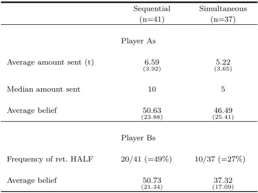
[image:13.595.163.429.272.471.2]Table 1 provides a summary of subjects’ behavior. Overall, we observe that the investment levels as well as A players’ beliefs are both slightly higher in SEQ than in SIM. When it comes to B players the difference is more substantial as B players share almost twice as much in SEQ than in SIM.
Table 1
Summary of subject behavior
Sequential Simultaneous (n=41) (n=37)
Player As
Average amount sent (t) 6.59
(3.92) (35.22.65)
Median amount sent 10 5
Average belief 50.63
(23.88) (2546.49.41)
Player Bs
Frequency of ret. HALF 20/41 (=49%) 10/37 (=27%)
Average belief 50.73
(21.34) (1737.32.09)
Note: Standard errors included in the parentheses.
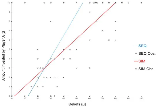
scattered (i.e., multiple As investing different amounts given the same belief).14
Figure 1
Relationship between beliefs and investment levels in SIM
While the conjecture that the sequential institutional design is more efficient seems compelling (due to the fact that the trustor can reveal a high level of trust and induce a high level of cooperation), our theoretical argument suggests that the comparison of the two institutions may not be trivial. Given that we observe a high variation in investment levels, this opens up the possibility that the simultaneous design could outperform the sequential one.
Main result:The efficiency of the sequential institution is higher than the efficiency of the simultaneous institution. The magnitude of the effect, however,
14This is indicative of and consistent with heterogeneity in risk-aversion levels. There are a
is only weakly significant.
[image:15.595.162.429.336.527.2]Support: The averaget sent by player A in SEQ and SIM is 6.59 and 5.22, respectively (a 26% increase in investment from SIM to SEQ). The two-sided Mann-Whitney test (adjusting for ties) indicates that the investment levels are significantly different at the 10% level (p=0.092). The average investment levels, suggesting mildly higher efficiency of the sequential institution, however, do not tell the entire story. The two institutions induce visibly different distributions of t. In SEQ the investments are more dispersed and pushed to the upper boundary, whereas in SIM they are more concentrated in the middle of the support (see Figure 2). The number of A players who sent the maximum amountt= 10 is higher in SEQ than in SIM (51.2% vs. 24.3%), but the number of those who sent nothing does not differ between treatments (12.2% vs. 10.8%). The Epps-Singleton test rejects the hypothesis that the distribution are generated by the same stochastic process (p=0.049).
Figure 2
Investment levels in SEQ and SIM
send the full amount. We therefore compare the realized payoffs of A players in SEQ and SIM which were respectively 10.44 and 6.89. The Mann-Whitney test reports that the difference is highly statistically significant (p=0.002).
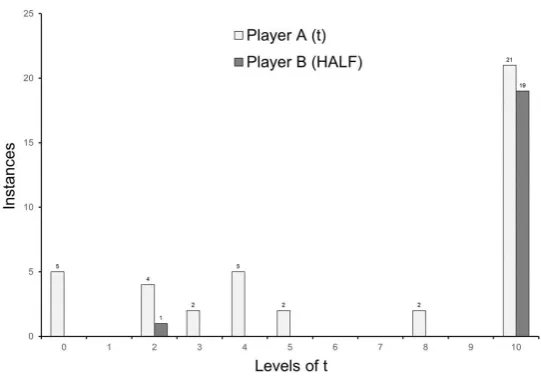
What about B players? Do they share more frequently when they receive a highert from A players in SEQ? Note that this analysis is meaningful only in SEQ where the choice oftis directly observed by B players before making their decisions.15
Observation 1:B players only reward the highest level of exposure.
Support: Figure 3 displays the distribution of decisions in SEQ. Bars labeled “A’s invested” present the number of instances in which A players sent a par-ticular t. The adjacent bars labeled “B’ returned HALF” show the number of instances in which B players returned HALF for a given t they received. It is clear from the figure that there is not an increasing relationship betweentsent by A’s and the frequency of HALF returned by B’s. Notice that among 41 pairs, 21 (51%) of the A players sentt= 10 and 19 (91%) of B players who received t= 10 returned HALF. On the other hand, only 1 out of the 20 B players (5%) who received t <10, returned HALF. Our data thus provide evidence that an increase intdoes not induce a higher frequency of returning HALF by B players. The above observation suggests that sending less than the maximum amount t <10 is interpreted by B players as being distrustful rather than trusting (e.g., as in Falk and Kosfeld, 2006; Schnedler and Vadovi˘c, 2011; see also Morita and Servátka, 2016 and 2018) and leads to a severe reduction in cooperation. Bolton, Brandts, and Ockenfels (1998), Charness and Rabin (2002), and Song (2008) also reject strictly monotone relationship between player A’s exposure and player B’s response. Some non–strict-monotonicity is also observed in the original Berget al.(1995) study as well as in Ortmann, Fitzgerald, and Boeing (2000) and Rigdon (2009); however, it is not as extreme as in our experiment.
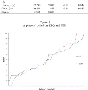
At last we compare A players’ beliefs between the two institutions (presented in Figure 4). We have elicited beliefs over actions (returning ZERO or HALF) rather than strategies of player B. In SIM, B players’ strategies coincide with their actions, but in SEQ this is not the case. There, a strategy is a function mapping investment levels into probabilities of sharing. It would be complicated and quite impractical trying to elicit subjects’ full belief function, so instead we opted for a simpler measure over the action space. This still gives us the same idea about what A players in SEQ think about the possible sharing rate by B players. It is this interpretation that we have in mind when comparing A players’ elicited beliefs and formulating the following observation.
Observation 2:While beliefs of A players about B players’ sharing rate do
15For illustration, when player A sent t = 10 in SIM, only 1 out of 9 (11%) B players
Figure 3
Instances of decisions in SEQ
not differ between the two institutions, the average investmenttconditional on player’s A belief is greater in SEQ than in SIM.
Support:The comparison of beliefs in the two treatments is presented in Fig-ure 4. The average belief of A players in SEQ and SIM is 50.63 and 46.49, re-spectively. While the belief in SEQ is somewhat higher, the Mann-Whitney test indicates that the difference is statistically insignificant (p= 0.527; two-sided). However, what differs significantly between the institutions is the relationship betweent’s and elicited beliefsµ. We compare the slopes of regressions oft on beliefs in SEQ and SIM treatments. The Tobit analysis of pooled players’ A decisions based on the treatment they participated in has the form:
ti=α+β1µi+β2TSEQµi+γTSEQ+ǫi
whereTSEQrepresents a dummy variable that equals 1 for SEQ treatment and
Table 2
Tobit regression estimates for SEQ vs. SIM
Coef. Std. Err. t-value p > t A’s beliefs (β1) 0.128 0.036 3.55 0.001
A’s beliefs × Dum. (β2)
0.109 0.058 1.89 0.063 Dummy (γ) -2.748 2.813 -0.98 0.332 Cons. (α) -0.248 1.829 -0.14 0.893 Sigma 4.883 0.623
Figure 4
A players’ beliefs in SEQ and SIM
5 Discussion
[image:18.595.153.435.177.466.2]The argument is based on the fact that the former institutional design allows the trustor to display trust before the trustee takes an action. While this argu-ment seems intuitive, we theoretically show that under certain circumstances the simultaneous institution might be more efficient. We also compare the two institutional designs experimentally and find that the sequential institution is more efficient; however, this increase in efficiency is only weakly statistically significant and perhaps not as dramatic as one would have intuitively expected. The sequential institution elicits a steeper relationship between the beliefs of A players and their investment levels than the simultaneous one. Interestingly, we also find that it is necessary for the trustor to place complete trust in the trustee in order for this trust to be reciprocated. It seems that trustees re-ward only what they consider to be absolute trust and appear to interpret any investment smaller than the maximum possible as a sign of distrust.16
Our results are relevant from a theoretical standpoint and also from the point of view of designing institutions. In practice, institutions have evolved to incor-porate various features to make market interactions safer. Most real-life business deals have a sequential structure, which however is heavily reinforced through systems allowing credible reputation building and third-party enforcement (e.g. contracts). In our daily lives we commonly experience sequential exchange. For example, a university first charges tuition and only then delivers classes; a con-tractor typically first fixes your deck, before collecting the payment; a utility provider delivers a month of service before sending out a bill.
One of the prototypical examples of simultaneous exchange is paying money for a ransom - a situation well-known from blockbuster movies. In cases where formal institutions can offer only limited security, business dealings tend to grav-itate toward simultaneous form of exchange. For instance, transactions facili-tated by online marketplaces, such as Craigslist, typically display some features of simultaneous exchange. Buying a used car from a private seller involves meet-ing up at a mutually agreeable spot (e.g. DMV), where the payment collection and signing over the title occurs simultaneously. Another interesting example are transactions in cryptocurrencies. With Bitcoin for instance, there is a some delay between the payment authorization and (a reasonable degree of) confir-mation, i.e. the transaction needs to be added to the ledger and covered with several additional blocks. This time interval may be exploited by tricksters and scammers for purposes of double-paying. It is therefore advisable that parties wait for a sufficient confirmation before exchanging the product.
It is virtually impossible to find real life examples that would directly corre-spond to our experimental environment; nor was this an objective of our study to try to replicate such instances. Instead, we aimed to isolate the role of trust in a simple situation of exchange between two parties. Our main contribution
16The result that trustees almost exclusively share following the maximum investment may
create the impression that our theoretical assumption of strict monotone relationship between the investment level and the probability of equal split (p′(t)> 0) is rejected by the data.
to the literature stems from varying the information available to the trustee about the trustor’s decision. In terms of our findings, similarly to Clark and Sefton (2001), who studied behavior in a sequential prisoner’s dilemma, we also observe that when interaction is sequential, more transactions are initiated and completed. Thus, the sequential design has the potential to increase the overall welfare while making it also profitable for the trusting party. Hence, our ex-periment advocates carefully designing institutions that allow for a display of trusting behavior.
Laboratory experiments are a powerful tool for comparing and evaluating the performance of institutions, studying their allocative and distributive proper-ties, and exploring their behavioral limitations (Smith, 1982 and 1994; see also Servátka, 2018). Supressing many realistic features allows for a tight control of the decision-making environment. At the same time, the laboratory results are to be interpreted with caution as they may not necessarily generalize into dif-ferent strategic and contextual environments in which the interaction between transacting parties might be embedded. For example, while in the experiment subjects were assigned to roles at random, in certain environments of everyday life there could be a selection of opportunistic types into the role of the second mover. In that case the market could eventually fail irrespective of whether de-cisions are sequential or simultaneous. We therefore consider further laboratory experiments varying the underlying environment as well as field experimenta-tion to be fruitful avenues for future research on the empirical relevance of the sequential versus simultaneous design.
Appendix A: Deriving a Sharing Response Function
B Players face a simple choice (denoted by S), they may either defect (i.e. S=D) or cooperate (i.e. S=C). We assume that players of type B feel some form of guilt or remorse when betraying the trust of players of type A, that is when they playD. The utility of playeriis
(A1) u(Si;t) =
(
3t−giv(t) ifSi=D
3t/2 ifSi=C,
where gi >0 is the “guilt” parameter andv(t) is a strictly increasing, strictly
convex function with v(0) = 0. The greater the expected trust displayed by players of type A, the greater the guilt of not reciprocating. We assume that B players have the same utility in the simultaneous as in the sequential case, but that it depends in the former on the average (or expected) trustt, whereas in the latter the actual decision is observable and t=t. B players are all the same, but differ in their guilt parametergi, which is distributed on the interval
[0,∞) according to the cumulative distribution function F(g), withF′(g)>0.
doing so, i.e. if
(A2) 1.5t≥giv(t).
When trust is zero, any player will defect. The higher the trust / the investment
t, the lower is the cutoff ˜g for which ˜g = 1.5t/v(t), because v(t) is strictly convex. Since F′(g) >0, a higher t by A players will thus result in a strictly
higher probability of sharing by players of type B. Note that the probability of sharing is not restricted in any way beyond p′ >0, since we have not made
any further assumptions on the distribution of g and the shape of v. This is obviously but one example of how one can derive the sharing response function that we had postulated in our model, and there are many potential alternative modeling assumptions which yield the same type of response function.
Appendix B: Instructions
The player type and ID number are stated at the top of each page of instruc-tions and on each decision form, as follows:
You are a Player ____ ID#:____
B.1 GENERAL INSTRUCTIONS
This is an experiment studying decision-making. The instructions are simple and if you follow them carefully and make good decisions, you might earn a considerable amount of money which will be paid to you in cash at the end of the experiment. It is therefore very important that you read these instructions with care.
No Talking Allowed
It is prohibited to communicate with other participants during the experi-ment. Should you have any questions please ask us. If you violate this rule, we shall have to exclude you from the experiment and from all payments.
Anonymity
Each person will be randomly matched with another person in the experiment. No one will learn the identity of the person she/he is matched with. You will be matched with the same person for the entire experiment.
Types
Each two person group will consist of two types of participants (Player A and Player B) that are assigned randomly. Your assigned type will be listed at the top of each task instruction sheet.
The Game
You are randomly paired with another individual. One member of your pair will be a player A and the other one will be player B. Find your type in the upper right corner of this sheet. You will never be able to find out the identity of the player you are paired with.
(a) Player A begins the process with $10, and player B begins with $0. (b) Player A then has the opportunity to transfer all, any portion, or none of his/her $10 to player B. Player A circles his or her decision on line (1) of the attached Decision Sheet. The amount that is not transferred is player A’s to keep. The amount that player A transfers triples when it reaches player B. For example, if A transfers $10 to B, B receives $30. If A transfers $5 to B, B receives $15. If A transfers $0 to B, B receives $0.
(c) Player B then has the opportunity to transfer half or none of the money he/she has received to player A. Player B indicates his/her decision in line (3) of the Decision Sheet by circling eitherHALForZERO. The amount that is not transferred is player B’s to keep, and the amount transferred is added to player A’s earnings.
B.2 Task 1 Instructions for Player A [SIM]
In task 2, the initially described two stage game is played simultaneously. That is, player A makes their transfer decision at the same time that player B makes their transfer decision back to player A. Therefore, player B is going to make their decisionwithout knowing how much player A has transferred to them.
For task 1, you must answer the following question:
Without knowing how much player A has transferred to them, what is the percentage of players B in the room that will return HALF of the amount that they receive, i.e. HALF of the tripled amount that is transferred to them from player A counterpart?
Your payout will depend on your accuracy. The payout is calculated as follows: You will start with $5. For every percentage point (1 % point) of mistake, 10 cents will be deducted from this $5. The mistake is the absolute value of (your answer – the actual percentage). For example, if you answer accurately, you will get $5. If you miss by 20% points (i.e., your answer is either twenty percentage points too high or twenty percentage points too low), you will be paid $3 (500 - 20 x 10 = 300). If your mistake will be larger than or equal to 50% points, then your earnings from this task will be zero.
I believe that ... % of players B in the room will return HALF of the tripled amount.
B.3 Task 1 Instructions for Player B
In task 2, the initially described two stage game is played simultaneously. That is, player A makes their transfer decision at the same time that player B makes their transfer decision back to player A. Therefore, player B is going to make their decision without knowing how much player A has transferred to them.
Without knowing how much player A has transferred to them, what is the percentage of players B in the room that will return HALF of the amount that they receive, i.e. HALF of the tripled amount that is transferred to them from player A counterpart?
For task 1, please answer the following question:
What is the average answer of players A in the room to question posed to them above?
Your payout will depend on your accuracy. The payout is calculated as follows: You will start with $5. For every percentage point (1 % point) of mistake, 10 cents will be deducted from this $5. The mistake is the absolute value of (your answer – the actual percentage). For example, if you answer accurately, you will get $5. If you miss by 20% points (i.e., your answer is either twenty percentage points too high or twenty percentage points too low), you will be paid $3 (500 - 20 x 10 = 300). If your mistake will be larger than or equal to 50% points, then your earnings from this task will be zero.
I believe that the average answer of players A was ... %.
B.4 Task 2 DECISION SHEET
Player A begins with $10. Player B begins with $0.
Each dollar that Player A gives to Player B is multiplied by 3 by the experi-menter.
The decisions of both players will be made simultaneously. Therefore, player Bwill not know how much player A has transferred to player B before player B makes their decision of whether to return HALF or ZERO.
(1) Player A’s decision:
Circle the amount that you want to transfer to player B
0 1 2 3 4 5 6 7 8 9 10
(2) Player B’s decision:
Circle the amount you want to transfer to player A: HALF or ZERO
(3) Experimenter calculates total earnings:
Final payoff to player A:___________________ Final payoff to player B: ___________________
B.5 Task 1 Instructions for Player A [SEQ]
In task 2, the initially described two stage game is playedsequentially. That is, player A makes their transfer decision and then player B makes their transfer decision after being able to see how much player A transferred to them. There-fore, player B is going to make their decisionknowinghow much player A has transferred to them.
For task 1, you must answer the following question:
is the percentage of players B in the room that will return HALF of the amount that they receive, i.e. HALF of the tripled amount that is transferred to them from player A counterpart?
Your payout will depend on your accuracy. The payout is calculated as follows: You will start with $5. For every percentage point (1 % point) of mistake, 10 cents will be deducted from this $5. The mistake is the absolute value of (your answer – the actual percentage). For example, if you answer accurately, you will get $5. If you miss by 20% points (i.e., your answer is either twenty percentage points too high or twenty percentage points too low), you will be paid $3 (500 - 20 x 10 = 300). If your mistake will be larger than or equal to 50% points, then your earnings from this task will be zero.
I believe that ... % of players B in the room will return HALF of the tripled amount.
B.6 Task 1 Instructions for Player B
In task 2, the initially described two stage game is playedsequentially. That is, player A makes their transfer decision and then player B makes their transfer decision after being able to see how much player A transferred to them. There-fore, player B is going to make their decisionknowinghow much player A has transferred to them.
Type A players in task 1 are asked to answer the following question:
After seeing how much is transferred to them from player A, what is the percentage of players B in the room that will return HALF of the amount that they receive, i.e. HALF of the tripled amount that is transferred to them from player A counterpart?
For task 1, please answer the following question:
What is the average answer of players A in the room to question posed to them above?
Your payout will depend on your accuracy. The payout is calculated as follows: You will start with $5. For every percentage point (1 % point) of mistake, 10 cents will be deducted from this $5. The mistake is the absolute value of (your answer – the actual percentage). For example, if you answer accurately, you will get $5. If you miss by 20% points (i.e., your answer is either twenty percentage points too high or twenty percentage points too low), you will be paid $3 (500 - 20 x 10 = 300). If your mistake will be larger than or equal to 50% points, then your earnings from this task will be zero.
I believe that the average answer of players A was ... %.
B.7 Task 2 DECISION SHEET
Player A begins with $10. Player B begins with $0.
The decisions of both players will be made sequentially. Therefore, player B willknowhow much player A has transferred to player B before player B makes their decision of whether to return HALF or ZERO.
(1) Player A’s decision:
Circle the amount that you want to transfer to player B
0 1 2 3 4 5 6 7 8 9 10
(2) Player B’s decision:
Circle the amount you want to transfer to player A: HALF or ZERO
(3) Experimenter calculates total earnings:
Final payoff to player A:___________________ Final payoff to player B: ___________________
References
[1] Ahn TK, Lee M, Ruttan L, Walker J (2007), “Asymmetric payoffs in simultaneous and sequential prisoner’s dilemma games,”Public Choice,132, pp. 353–366. [2] Andersen S, Harrison GW, Lau MI, Rutström EE (2008), “Eliciting risk and time
preferences,”Econometrica, 76(3), pp. 583–618.
[3] Arrow KJ (1976),The Limits of Organization, New York: Norton.
[4] Ashraf, N, Bohnet I, and Piankov N (2006), “Decomposing Trust and Trustworthi-ness,” Experimental Economics, Special Issue on Behavioral Economics, 9(3), pp. 193–208.
[5] Battigalli P and Dufwenberg M (2007), “Guilt in Games,” American Economic Review, Papers and Proceedings, 97, pp. 170–176.
[6] Ben-Ner A, Putterman L (2009), “Trust, communication and contracts: An exper-iment,”Journal of Economic Behavior &Organization, 70(1-2), pp. 106–121. [7] Ben-Ner A, Putterman L, Ren T (2011), “Lavish returns on cheap talk: Two-way
communication in trust games,”Journal of Socio-Economics,40(1), pp. 1–3. [8] Berg J, Dickhaut J, and McCabe K (1995), “Trust, Reciprocity, and Social
His-tory,”Games&Economic Behavior, 10(1), pp. 122–142.
[9] Bolton G, Brandts J, and Ockenfels A (1998), “Measuring Motivations for the Reciprocal Responses Observed in a Simple Dilemma Game,” Experimental Eco-nomics, 1, pp. 207–219.
[10] Bracht J, Feltovich N (2008), “Efficiency in the trust game: an experimental study of precommitment,”International Journal of Game Theory, 37(1), pp. 39–72. [11] Bracht J, Feltovich N (2009), “Whatever you say, your reputation precedes you:
Observation and cheap talk in the trust game,”Journal of Public Economics, 93(9-10), pp. 1036–1044.
[12] Brandts J and Charness G (2000), “Hot and Cold Decisions and Reciprocity in Experiments with Sequential Games,”Experimental Economics, 2(3), pp. 227–238. [13] Brandts J and Charness G (2011), “The strategy versus the direct-response method: a first survey of experimental comparisons,” Experimental Economics, 14(3), pp. 375–398.
[15] Camerer C (2003),Behavioral Game Theory: Experiments in Strategic Interac-tion, Princeton University Press.
[16] Casari, M. and T. N. Cason (2009), “The Strategy Method Lowers Measured Trustworthy Behavior,”Economics Letters, 103, pp. 157–159.
[17] Chaudhuri A, Gangadharan L (2007), “An experimental analysis of trust and trustworthiness,”Southern Economic Journal, pp. 959–985.
[18] Charness G, Cobo-Reyes R, and Jimenez N (2008), “An Investment Game with Third Party Intervention,”Journal of Economic Behavior&Organization, 68, pp. 18–28.
[19] Charness G, Kuhn P (2011), “Lab labor: What can labor economists learn from the lab?” InHandbook of Labor Economics, 4, pp. 229–330.
[20] Charness G and Rabin M (2002), “Understanding Social Preferences with Simple Tests,”Quarterly Journal of Economics, 74(6), pp. 1579–1601.
[21] Charness G and Dufwenberg M (2006), “Promises and Partnership,” Economet-rica, 117, pp. 817–869.
[22] Charness G, Dufwenberg M (2010), “Bare promises: An experiment,”Economics Letters, 107(2), pp. 281–283.
[23] Clark K and Sefton M (2001), “The Sequential Prisoner’s Dilemma: Evidence on Reciprocation,”Economic Journal, 111, pp. 51–68.
[24] Cooper DJ and Van Huyck JB (2003), “Evidence on the Equivalence of the Strate-gic and Extensive Form Representation of Games,”Journal of Economic Theory, 110, pp. 290–308.
[25] Cox JC (2004), “How to Identify Trust and Reciprocity,” Games & Economic Behavior, 46, pp. 260–281.
[26] Cox, JC and Deck CA (2005), “On the Nature of Reciprocal Motives,”Economic Inquiry, 43(3), pp. 623–635.
[27] Cox JC, Friedman D, and Gjerstad S (2007), “A Tractable Model of Reciprocity and Fairness,”Games&Economic Behavior, 59, pp. 17–45.
[28] Cox JC, Friedman D, and Sadiraj V (2008), “Revealed altruism,”Econometrica, 76(1), pp. 31–69.
[29] Cox JC, Kerschbamer R, and Neururer D (2016), “What is trustworthiness and what drives it?”Games&Economic Behavior, 98, pp. 197–218.
[30] Cox JC, Roberson B, Smith VL (1982), “Theory and behavior of single object auctions,”Research in Experimental Economics, 2(1), pp. 1–43.
[31] Dasgupta P (2000), “Economic progress and the idea of social capital,” in Das-gupta, P. and Serageldin, I. (eds),Social Capital: A Multifaceted Perspective, Wash-ington, D.C.: World Bank.
[33] Deck C, Lee J, Reyes JA, Rosen CC (2013), “A failed attempt to explain within subject variation in risk taking behavior using domain specific risk attitudes,” Jour-nal of Economic Behavior&Organization, 87, pp. 1–24.
[33] Deck C, Servátka M, Tucker S (2013), “An examination of the effect of messages on cooperation under double-blind and single-blind payoff procedures,” Experimen-tal Economics, 16(4), pp. 597–607.
[34] Dufwenberg M and Gneezy U (2000), “Measuring Beliefs in an Experimental Lost Wallet ”Games&Economic Behavior, 30, pp. 163–182.
[35] Dufwenberg M (2002), “Marital investments, time consistency and emotions,”
[36] Dufwenberg M and Kirchsteiger G (2004), “A Theory of Sequential Reciprocity,”
Games&Economic Behavior, 47, pp. 268–98.
[37] Dufwenberg M, Servátka M, Vadovi˘c R (2017), “Honesty and informal agree-ments,”Games&Economic Behavior, 102, pp. 269–285.
[38] Eckel CC, Wilson RK (2004), “Is trust a risky decision?,”Journal of Economic Behavior&Organization, 55(4), pp. 447–465.
[39] Ellingsen T and Johannesson M (2008), “Pride and Prejudice: The Human Side of Incentive Theory,”American Economic Review, 98(3), pp. 990–1008.
[40] Engle-Warnick J and Slonim RL (2004), “The evolution of strategies in a repeated trust game,”Journal of Economic Behavior&Organization, 55(4), pp. 553–573. [41] Fairley K, Sanfey A, Vyrastekova J, Weitzel U (2016), “Trust and risk revisited,”
Journal of Economic Psychology, 57, pp. 74–85.
[42] Falk A, Fehr E, and Fischbacher U (2003), “On the Nature of Fair Behavior,”
Economic Inquiry, 41(1), pp. 20–26.
[44] Falk A and Fischbacher U (2006), “A Theory of Reciprocity,”Games&Economic Behavior, 54, pp. 293–315.
[44] Falk A and Kosfeld M (2006), “The Hidden Costs of Control,” American Eco-nomic Review, 96(5), pp. 1611–1630.
[45] Fehr E (2009), “On the economics and biology of trust,”Journal of the European Economic Association, 7(23), pp. 235–266.
[46] Fehr E and Schmidt KM (1999), “A theory of fairness, competition, and cooper-ation,”Quarterly Journal of Economics, 114(3), pp. 817–868.
[47] Fukuyama F (1995), Trust: The Social Virtues and the Creation of Prosperity,
New York: Free Press.
[48] Güth, W, Huck S, and Mueller W (2001), “The Relevance of Equal Splits in Ultimatum Games,”Games&Economic Behavior, 37, pp. 161–169.
[49] Gneezy U, Leonard KL, List JA (2009), “Gender differences in competition: Evi-dence from a matrilineal and a patriarchal society,”Econometrica, 77(5), pp. 1637– 1664.
[50] Henrich J, Boyd R, Bowles S, Camerer C, Fehr E, Gintis H, McElreath R (2001), “In search of homo economicus: behavioral experiments in 15 small-scale societies,”
American Economic Review, 91(2), pp. 73–78.
[51] Holt CA, Laury SK (2002), “Risk aversion and incentive effects,”American Eco-nomic Review, 92(5), pp. 1644–1655.
[52] Houser D, Schunk D, Winter J (2010), “Distinguishing trust from risk: An anatomy of the investment,”Journal of Economic Behavior&Organization, 74(1-2), pp. 72–81.
[53] Houser D, Xiao E (2015), “House money effects on trust and reciprocity,”Public Choice, 163(1-2), pp. 187–199.
[54] Huck S, Mueller W and Normann H-T (2011), “Stackelberg Beats Cournot — On Collusion and Efficiency in Experimental Markets,”Economic Journal, 111, 474, pp. 749–765.
[55] Huck S, Lünser GK, Tyran JR (2012), “Competition fosters trust,” Games &
Economic Behavior, 76(1), pp. 195–209.
[57] Knack S and Keefer P (1997), “Does Social Capital Have an Economic Payoff? A Cross-Country Investigation,”Quarterly Journal of Economics, 112, pp. 1251–1288. [58] La Porta R, Lopez-de-Salanes F, Shleifer A, and Vishny R (1997), “Trust in Large Organizations,”American Economic Review Papers&Proceedings, 87, pp. 333–338. [59] Levine DK (1998), “Modeling altruism and spitefulness in experiments,”Review
of Economic Dynamics, 1(3), pp. 593–622.
[60] McCabe K, Smith V, and LePore M (2000), “Intentionality detection and min-dreading: Why does game form matter?” Proceedings of the National Academy of Sciences of the United States of America, 97(8), pp. 4404–4409.
[61] Morita H and Servátka M (2016), “Does Group Identity Prevent Inefficient In-vestment in Outside Options? An Experimental Investigation,” in S.J. Goerg and J. Hamman eds.,Research in Experimental Economics: Experiments in Organizational Economics, 19, pp. 105–127.
[62] Morita H and Servátka M (2018), “Investment in Outside Options as Opportunis-tic Behavior: An Experimental Investigation,” Southern Economic Journal, 85, pp. 457–484.
[63] Ortmann A, Fitzgerald J, and Boeing C (2000), “Trust, Reciprocity, and Social History: A Re-examination,”Experimental Economics, 3(3), pp. 81–100.
[Ostrom1992] Ostrom E, Walker J, and Gardner R, “Covenants With and Without a Sword: Self-Governance is Possible,”American Political Science Review, 86, pp. 404–417.
[65] Putnam R (1993), Making Democracy Work: Civic Traditions in Modem Italy, Princeton: Princeton University Press.
[66] Rigdon M (2009), “Trust and reciprocity in incentive contracting,” Journal of Economic Behavior &Organization, 70(1-2), pp. 93–105.
[67] Schlag KH, Tremewan J, Van der Weele JJ (2015), “A penny for your thoughts: A survey of methods for eliciting beliefs,”Experimental Economics, 18(3), pp. 457– 490.
[68] Schnedler W and Vadovi˘c R (2011), “Legitimacy of Control,” Journal of Eco-nomics &Management Strategy, 20(4), pp. 985–1009.
[69] Schotter A, Weiss A, and Zapater I (1996), “Fairness and Survival in Ultimatum and Dictatorship Games,” Journal of Economic Behavior & Organization, 31(1), pp. 37–56.
[70] Servátka M (2018), “How Do Experiments Inform Collective Action Research?”
Research Agenda for New Institutional Economics, C. Ménard & M. Shirley eds., Edward Elgar Publishing, pp. 260–268.
[71] Servátka M, Tucker S, Vadovi˘c R (2011), “Building trust - one gift at a time,”
Games, 2(4), pp. 412–433.
[72] Servátka M, Tucker S, Vadovi˘c R, “Words speak louder than money,”Journal of Economic Psychology, 32(5), pp. 700–709.
[73] Sheremeta RM, Zhang J (2014), “Three-Player Trust Game with Insider Com-munication,”Economic Inquiry, 52(2), pp. 576–591.
[74] Smith VL (1962), “An experimental study of competitive market behavior,” Jour-nal of Political Economy, 70(2), pp. 111–137.
[76] Smith VL (1982), “Microeconomic systems as an experimental,” American Eco-nomic Review, 72(5), pp. 923–955.
[77] Smith VL (1994), “Economics in the Laboratory,”Journal of Economic Perspec-tives, 8(1), pp. 113–131.
[78] Song F (2008), “Trust and Reciprocity Behavior and Behavioral Forecasts: In-dividuals versus Group-Representatives,”Games&Economic Behavior, 62(2), pp. 675–696.
[79] Woods D, Servátka M (2016), “Testing psychological forward induction and the updating of beliefs in the lost wallet game,”Journal of Economic Psychology, 56, pp. 116–125.
[80] Zak P and Knack S (2001), “Trust and Growth,” Economic Journal, 111(470), pp. 295–321.
Till Gross
Department of Economics, D-897 Loeb, Carleton University, 1125 Colonel By Drive, Ottawa, ON, K1S 5B6
Maro˘s Servátka
MGSM Experimental Economics Lab-oratory, Macquarie Graduate School of Management, 99 Talavera Rd., North Ryde NSW 2113, Australia
[email protected] Radovan Vadovi˘c
Department of Economics, D-897 Loeb, Carleton University, 1125 Colonel By Drive, Ottawa, ON, K1S 5B6