Proceedings of the 57th Annual Meeting of the Association for Computational Linguistics, pages 2963–2977 2963
Interpretable Neural Predictions with Differentiable Binary Variables
Joost Bastings ILLC
University of Amsterdam [email protected]
Wilker Aziz ILLC
University of Amsterdam [email protected]
Ivan Titov
ILLC, University of Amsterdam ILCC, University of Edinburgh
Abstract
The success of neural networks comes hand in hand with a desire for more interpretabil-ity. We focus on text classifiers and make them more interpretable by having them provide a justification—arationale—for their predic-tions. We approach this problem by jointly training two neural network models: a latent model that selects a rationale (i.e. a short and informative part of the input text), and a classifier that learns from the words in the rationale alone. Previous work proposed to assign binary latent masks to input positions and to promote short selections via sparsity-inducing penalties such as L0 regularisation. We propose a latent model that mixes discrete and continuous behaviour allowing at the same time for binary selections and gradient-based training without REINFORCE. In our formu-lation, we can tractably compute the expected value of penalties such asL0, which allows us to directly optimise the model towards a pre-specified text selection rate. We show that our approach is competitive with previous work on rationale extraction, and explore further uses in attention mechanisms.
1 Introduction
Neural networks are bringing incredible perfor-mance gains on text classification tasks (Howard and Ruder, 2018; Peters et al., 2018; Devlin et al.,2019). However, this power comes hand in hand with a desire for more interpretability, even though its definition may differ (Lipton, 2016). While it is useful to obtain high classification accuracy, with more data available than ever before it also becomes increasingly important to justify predictions. Imagine having to classify a large collection of documents, while verifying that the classifications make sense. It would be extremely time-consuming to read each document to evaluate the results. Moreover, if we do not
pours a dark amber color with decent head that does not recede much . it ’s a tad too dark to see the carbonation , but fairs well . smells of roasted malts
and mouthfeel is quite strong in the sense that you can get a good taste of it before you even swallow .
Rationale Extractor
poursa dark amber color with decent headthat does not recede much . it ’sa tad too dark to see the carbonation , but fairs well .smells of roasted malts and mouthfeel is quite strong in the sense that you can get a good taste of it before you even swallow .
[image:1.595.323.507.218.383.2]Classifier look:FFFF
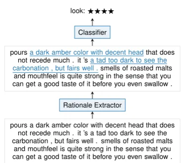
Figure 1: Rationale extraction for a beer review.
know why a prediction was made, we do not know if we can trust it.
What if the model could provide us the most important parts of the document, as a justification for its prediction? That is exactly the focus of this paper. We use a setting that was pioneered byLei et al.(2016). Arationaleis defined to be a short yetsufficientpart of the input text; short so that it makes clear what is most important, and sufficient so that a correct prediction can be made from the rationale alone. One neural network learns to ex-tract the rationale, while another neural network, with separate parameters, learns to make a predic-tion from just the rapredic-tionale. Lei et al. model this by assigning a binary Bernoulli variable to each input word. The rationale then consists of all the words for which a 1 was sampled. Because gradi-ents do not flow through discrete samples, the ra-tionale extractor is optimized using REINFORCE (Williams, 1992). An L0 regularizer is used to
make sure the rationale is short.
repa-rameterization of a random variable that exhibits both continuous and discrete behavior (Louizos et al., 2017). To promote compact rationales, we employ a relaxed form of L0 regularization
(Louizos et al.,2017), penalizing the objective as a function of the expected proportion of selected text. We also propose the use of Lagrangian re-laxation to target a specific rate of selected input text.
Our contributions are summarized as follows:1
1. we present a differentiable approach to ex-tractive rationales (§2) including an objective that allows for specifying how much text is to be extracted (§4);
2. we introduce HardKuma (§3), which gives support to binary outcomes and allows for reparameterized gradient estimates;
3. we empirically show that our approach is competitive with previous work and that HardKuma has further applications, e.g. in attention mechanisms. (§6).
2 Latent Rationale
We are interested in making NN-based text clas-sifiers interpretable by (i) uncovering which parts of the input text contribute features for classifica-tion, and (ii) basing decisions on only a fraction of the input text (a rationale). Lei et al. (2016) approached (i) by inducing binary latent selectors that control which input positions are available to an NN encoder that learns features for classifica-tion/regression, and (ii) by regularising their archi-tectures using sparsity-inducing penalties on latent assignments. In this section we put their approach under a probabilistic light, and this will then more naturally lead to our proposed method.
In text classification, an input xis mapped to a distribution over target labels:
Y|x∼Cat(f(x;θ)), (1)
where we have a neural network architecture f(·;θ)parameterize the model—θcollectively de-notes the parameters of the NN layers inf. That is, an NN maps from data space (e.g. sentences, short paragraphs, or premise-hypothesis pairs) to the categorical parameter space (i.e. a vector of class probabilities). For the sake of concreteness,
1Code available at https://github.com/
bastings/interpretable_predictions.
consider the input a sequence x = hx1, . . . , xni.
A targetyis typically a categorical outcome, such as a sentiment class or an entailment decision, but with an appropriate choice of likelihood it could also be a numerical score (continuous or integer).
Lei et al. (2016) augment this model with a collection of latent variables which we denote by z=hz1, . . . , zni. These variables are responsible
for regulating which portions of the input x con-tribute with predictors (i.e. features) to the clas-sifier. The model formulation changes as follows:
Zi|x∼Bern(gi(x;φ))
Y|x, z∼Cat(f(xz;θ)) (2)
where an NN g(·;φ) predicts a sequence of n Bernoulli parameters—one per latent variable— and the classifier is modified such thatziindicates
whether or not xi is available for encoding. We
can think of the sequence z as a binary gating mechanism used to select a rationale, which with some abuse of notation we denote byxz. Figure 1illustrates the approach.
Parameter estimation for this model can be done by maximizing a lower boundE(φ, θ)on the log-likelihood of the data derived by application of Jensen’s inequality:2
logP(y|x) = logEP(z|x,φ)[P(y|x, z, θ)]
JI
≥EP(z|x,φ)[logP(y|x, z, θ)] =E(φ, θ).
(3)
These latent rationales approach the first objec-tive, namely, uncovering which parts of the input text contribute towards a decision. However note that an NN controls the Bernoulli parameters, thus nothing prevents this NN from selecting the whole of the input, thus defaulting to a standard text clas-sifier. To promote compact rationales, Lei et al. (2016) impose sparsity-inducing penalties on la-tent selectors. They penalise for the total number of selected words,L0in (4), as well as, for the
to-tal number of transitions, fused lasso in (4), and approach the following optimization problem
min
φ,θ −E(φ, θ) +λ0
n
X
i=1
zi
| {z }
L0(z)
+λ1
n−1
X
i=1
|zi−zi+1|
| {z }
fused lasso
(4)
via gradient-based optimisation, whereλ0andλ1
are fixed hyperparameters. The objective is how-ever intractable to compute, the lowerbound, in
2This can be seen as variational inference (Jordan et al.,
particular, requires marginalization of O(2n) bi-nary sequences. For that reason,Lei et al. sam-ple latent assignments and work with gradient es-timates using REINFORCE (Williams,1992).
The key ingredients are, therefore, binary la-tent variables and sparsity-inducing regulariza-tion, and therefore the solution is marked by non-differentiability. We propose to replace Bernoulli variables by rectified continuous random variables (Socci et al.,1998), for they exhibit both discrete and continuous behaviour. Moreover, they are amenable to reparameterization in terms of a fixed random source (Kingma and Welling, 2014), in which case gradient estimation is possible without REINFORCE. Following Louizos et al. (2017), we exploit one such distribution to relaxL0
reg-ularization and thus promote compact rationales with a differentiable objective. In section3, we in-troduce this distribution and present its properties. In section4, we employ a Lagrangian relaxation to automatically target a pre-specified selection rate. And finally, in section5we present an example for sentiment classification.
3 Hard Kumaraswamy Distribution
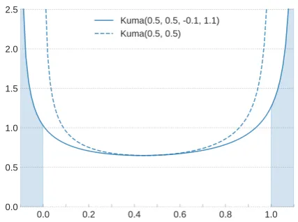
Key to our model is a novel distribution that ex-hibits both continuous and discrete behaviour, in this section we introduce it. With non-negligible probability, samples from this distribution evalu-ate to exactly 0 or exactly 1. In a nutshell: i) we start from a distribution over the open inter-val (0,1)(see dashed curve in Figure 2); ii) we then stretch its support from l < 0 tor > 1 in order to include {0} and {1} (see solid curve in Figure2); finally, iii) we collapse the probability mass over the interval(l,0]to{0}, and similarly, the probability mass over the interval[1, r)to{1} (shaded areas in Figure2). Thisstretch-and-rectify technique was proposed byLouizos et al.(2017), who rectified samples from the BinaryConcrete (or GumbelSoftmax) distribution (Maddison et al., 2017;Jang et al., 2017). We adapted their tech-nique to the Kumaraswamy distribution motivated by its close resemblance to a Beta distribution, for which we have stronger intuitions (for example, its two shape parameters transit rather naturally from unimodal to bimodal configurations of the distri-bution). In the following, we introduce this new distribution formally.3
3We use uppercase letters for random variables (e.g. K,
T, andH) and lowercase for assignments (e.g.k,t,h). For a
0.0 0.2 0.4 0.6 0.8 1.0 0.0
0.5 1.0 1.5 2.0 2.5
[image:3.595.309.523.64.223.2]Kuma(0.5, 0.5, 0.1, 1.1) Kuma(0.5, 0.5)
Figure 2: TheHardKumadistribution: we start from a Kuma(0.5,0.5), and stretch its support to the interval (−0.1,1.1), finally we collapse all mass before0to{0} and all mass after1to{1}.
3.1 Kumaraswamy distribution
The Kumaraswamy distribution (Kumaraswamy, 1980) is a two-parameters distribution over the openinterval(0,1), we denote a Kumaraswamy-distributed variable byK ∼ Kuma(a, b), where a ∈ R>0 andb ∈ R>0 control the distribution’s
shape. The dashed curve in Figure2illustrates the density of Kuma(0.5,0.5). For more details in-cluding its pdf and cdf, consult AppendixA.
The Kumaraswamy is a close relative of the Beta distribution, though not itself an exponential family, with a simple cdf whose inverse
FK−1(u;a, b) =
1−(1−u)1/b 1/a
, (5)
foru∈[0,1], can be used to obtain samples FK−1(U;α, β)∼Kuma(α, β) (6) by transformation of a uniform random source U ∼ U(0,1). We can use this fact to reparame-terize expectations (Nalisnick and Smyth,2016). 3.2 Rectified Kumaraswamy
We stretchthe support of the Kumaraswamy dis-tribution to include0and1. The resulting variable T ∼Kuma(a, b, l, r)takes on values in the open interval(l, r)wherel <0andr >1, with cdf
FT(t;a, b, l, r) =FK((t−l)/(r−l);a, b). (7)
We now define a rectified random variable, de-noted byH ∼ HardKuma(a, b, l, r), by passing
random variableK,fK(k;α)is the probability density
func-tion (pdf), condifunc-tioned on parametersα, andFK(k;α)is the
a sample T ∼ Kuma(a, b, l, r) through a hard-sigmoid, i.e. h = min(1,max(0, t)). The re-sulting variable is defined over the closed inter-val[0,1]. Note that while there is0probability of samplingt = 0, samplingh = 0corresponds to sampling any t ∈ (l,0], a set whose mass under
Kuma(t|a, b, l, r)is available in closed form:
P(H = 0) =FK
−l
r−l;a, b
. (8)
That is because all negative values of t are de-terministically mapped to zero. Similarly, sam-plest ∈[1, r)are all deterministically mapped to h= 1, whose total mass amounts to
P(H= 1) = 1−FK
1−l
r−l;a, b
. (9)
See Figure2 for an illustration, and AppendixA for the complete derivations.
3.3 Reparameterization and gradients
Because this rectified variable is built upon a Kumaraswamy, it admits a reparameterisation in terms of a uniform variable U ∼ U(0,1). We need to first sample a uniform variable in the open interval (0,1) and transform the result to a Ku-maraswamy variable via the inverse cdf (10a), then shift and scale the result to cover the stretched sup-port (10b), and finally, apply the rectifier in order to get a sample in the closed interval[0,1](10c).
k=FK−1(u;a, b) (10a) t=l+ (r−l)k (10b) h= min(1,max(0, t)), (10c)
We denote this h = s(u;a, b, l, r) for short. Note that this transformation has two discontinuity points, namely,t = 0 andt = 1. Though recall, the probability of samplingtexactly0or exactly1
is zero, which essentially means stochasticity cir-cumvents points of non-differentiability of the rec-tifier (see AppendixA.3).
4 Controlled Sparsity
Following Louizos et al. (2017), we relax non-differentiable penalties by computing them on ex-pectation under our latent modelp(z|x, φ). In ad-dition, we propose the use of Lagrangian relax-ation to target specific values for the penalties.
Thanks to the tractable Kumaraswamy cdf, the ex-pected value ofL0(z)is known in closed form
Ep(z|x)[L0(z)]
ind =
n
X
i=1
Ep(zi|x)[I[zi6= 0]]
= n
X
i=1
1−P(Zi= 0),
(11)
whereP(Zi = 0) =FK
−l
r−l;ai, bi
. This quan-tity is a tractable and differentiable function of the parameters φ of the latent model. We can also compute a relaxation of fused lasso by comput-ing the expected number of zero-to-nonzero and nonzero-to-zero changes:
Ep(z|x) "n−1
X
i=1
I[zi = 0, zi+16= 0] #
+Ep(z|x) "n−1
X
i=1
I[zi 6= 0, zi+1= 0] #
ind =
n−1
X
i=1
P(Zi = 0)(1−P(Zi+1 = 0))
+ (1−P(Zi = 0))P(Zi+1= 0).
(12)
In both cases, we make the assumption that latent variables are independent given x, in Appendix B.1.2we discuss how to estimate the regularizers for a modelp(zi|x, z<i)that conditions on the
pre-fixz<iof sampledHardKumaassignments.
We can use regularizers to promote sparsity, but just how much text will our final model se-lect? Ideally, we would target specific valuesrand solve a constrained optimization problem. In prac-tice, constrained optimisation is very challenging, thus we employ Lagrangian relaxation instead:
max
λ∈Rminφ,θ −E(φ, θ) +λ
>
(R(φ)−r) (13)
where R(φ) is a vector of regularisers, e.g. ex-pectedL0and expected fused lasso, andλis a
vec-tor of Lagrangian multipliersλ. Note how this dif-fers from the treatment ofLei et al.(2016) shown in (4) where regularizers are computed for as-signments, rather than on expectation, and where λ0, λ1 are fixed hyperparameters.
5 Sentiment Classification
5-way sentiment class (from very negative to very positive). The model consists of
Zi∼HardKuma(ai, bi, l, r)
Y|x, z∼Cat(f(xz;θ)) (14)
where the shape parameters a, b = g(x;φ), i.e. two sequences of n strictly positive scalars, are predicted by a NN, and the support boundaries
(l, r)are fixed hyperparameters.
We first specify an architecture that parameter-izes latent selectors and then use a reparameterized sample to restrict which parts of the input con-tribute encodings for classification:4
ei = emb(xi)
hn1 = birnn(en1;φr)
ui ∼ U(0,1)
ai=fa(hi;φa)
bi=fb(hi;φb)
zi=s(ui;ai, bi, l, r)
whereemb(·)is an embedding layer,birnn(·;φr)
is a bidirectional encoder, fa(·;φa) and fb(·;φb)
are feed-forward transformations with softplus
outputs, ands(·)turns the uniform sampleuiinto
the latent selector zi (see §3). We then use the
sampledzto modulate inputs to the classifier:
ei= emb(xi)
h(ifwd)= rnn(hi(−fwd1), ziei;θfwd)
h(ibwd)= rnn(hi(+1bwd), ziei;θbwd)
o=fo(h(nfwd),h(1bwd);θo)
where rnn(·;θfwd) and rnn(·;θbwd) are recurrent
cells such as LSTMs (Hochreiter and Schmidhu-ber, 1997) that process the sequence in different directions, andfo(·;θo)is a feed-forward
transfor-mation withsoftmaxoutput. Note howzi
modu-lates featuresei of the inputxi that are available
to the recurrent composition function.
We then obtain gradient estimates ofE(φ, θ)via Monte Carlo (MC) sampling from
E(φ, θ) =EU(0,I)[logP(y|x, sφ(u, x), θ)] (15)
where z = sφ(u, x) is a shorthand for
element-wise application of the transformation from uni-form samples to HardKuma samples. This repa-rameterisation is the key to gradient estimation through stochastic computation graphs (Kingma and Welling,2014;Rezende et al.,2014).
4We describe architectures using blocks denoted by layer(inputs;subset of parameters), boldface letters for vec-tors, and the shorthandvn
1 for a sequencehv1, . . . ,vni.
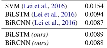
[image:5.595.329.501.63.141.2]SVM (Lei et al.,2016) 0.0154 BiLSTM (Lei et al.,2016) 0.0094 BiRCNN (Lei et al.,2016) 0.0087 BiLSTM(ours) 0.0089 BiRCNN(ours) 0.0088
Table 1: MSE on the BeerAdvocate test set.
Deterministic predictions. At test time we make predictions based on what is the most likely assignment for eachzi. Wearg maxacross
con-figurations of the distribution, namely, zi = 0,
zi = 1, or 0 < zi < 1. When the continuous
interval is more likely, we take the expected value of the underlying Kumaraswamy variable.
6 Experiments
We perform experiments on multi-aspect senti-ment analysis to compare with previous work, as well as experiments on sentiment classification and natural language inference. All models were implemented in PyTorch, and Appendix B pro-vides implementation details.
Goal. When rationalizing predictions, our goal is to perform as well as systems using the full input text, while using only a subset of the input text, leaving unnecessary words out for interpretability.
6.1 Multi-aspect Sentiment Analysis
In our first experiment we compare directly with previous work on rationalizing predictions (Lei et al.,2016). We replicate their setting.
Data. A pre-processed subset of the BeerAdvo-cate5 data set is used (McAuley et al., 2012). It consists of 220,000beer reviews, where multiple aspects (e.g. look, smell, taste) are rated. As shown in Figure1, a review typically consists of multiple sentences, and contains a 0-5 star rating (e.g. 3.5 stars) for each aspect. Lei et al. mapped the ratings to scalars in[0,1].
Model. We use the models described in §5with two small modifications: 1) since this is a regres-sion task, we use a sigmoid activation in the output layer of the classifier rather than a softmax,6 and
5
https://www.beeradvocate.com/
6From a likelihood learning point of view, we would have
assumed a Logit-Normal likelihood, however, to stay closer
Method
Look Smell Taste
% Precision % Selected % Precision % Selected % Precision % Selected
Attention (Lei et al.) 80.6 13 88.4 7 65.3 7
Bernoulli (Lei et al.) 96.3 14 95.1 7 80.2 7
Bernoulli(reimpl.) 94.8 13 95.1 7 80.5 7
[image:6.595.309.525.227.344.2]HardKuma 98.1 13 96.8 7 89.8 7
Table 2: Precision (% of selected words that was also annotated as the gold rationale) and selected (% of words not zeroed out) per aspect. In the attention baseline, the top 13% (7%) of words with highest attention weights are used for classification. Models were selected based on validation loss.
2) we use an extra RNN to conditionzionz<i:
ai=fa(hi,si−1;φa) (16a)
bi=fb(hi,si−1;φb) (16b)
si=rnn(hi, zi,si−1;φs) (16c)
For a fair comparison we followLei et al.by using RCNN7cells rather than LSTM cells for encoding sentences on this task. Since this cell is not widely used, we verified its performance in Table1. We observe that the BiRCNN performs on par with the BiLSTM (while using 50% fewer parameters), and similarly to previous results.
Evaluation. A test set with sentence-level ratio-nale annotations is available. Theprecisionof a ra-tionale is defined as the percentage of words with z6= 0that is part of the annotation. We also eval-uate the predictions made from the rationale using mean squared error (MSE).
Baselines. For our baseline we reimplemented the approach of Lei et al. (2016) which we call Bernoulliafter the distribution they use to sample z from. We also report their attention baseline, in which an attention score is computed for each word, after which it is simply thresholded to select the top-k percent as the rationale.
Results. Table2shows the precision and the per-centage of selected words for the first three as-pects. The models here have been selected based on validation MSE and were tuned to select a sim-ilar percentage of words (‘selected’). We observe that our Bernoulli reimplementation reaches the precision similar to previous work, doing a little bit worse for the ‘look’ aspect. Our HardKuma managed to get even higher precision, and it ex-tracted exactly the percentage of text that we
spec-7An RCNN cell can replace any LSTM cell and works
well on text classification problems. See appendixB.
0% 20% 40% 60% 80% 100%
Selected Text
0.008 0.009 0.010 0.011 0.012 0.013
MSE
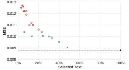
Figure 3: MSE of all aspects for various percentages of extracted text. HardKuma (blue crosses) has lower er-ror than Bernoulli (red circles; open circles taken from
Lei et al.(2016)) for similar amount of extracted text. The full-text baseline (black star) gets the best MSE.
ified (see §4).8 Figure3shows the MSE for all as-pects for various percentages of extracted text. We observe that HardKuma does better with a smaller percentage of text selected. The performance be-comes more similar as more text is selected.
6.2 Sentiment Classification
We also experiment on the Stanford Sentiment Treebank (SST) (Socher et al.,2013). There are 5 sentiment classes: very negative, negative, neutral, positive, and very positive. Here we use the Hard-Kuma model described in §5, a Bernoulli model trained with REINFORCE, as well as a BiLSTM.
Results. Figure4shows the classification accu-racy for various percentages of selected text. We observe that HardKuma outperforms the Bernoulli model at each percentage of selected text. Hard-Kuma reaches full-text baseline performance al-ready around 40% extracted text. At that point, it obtains atest score of 45.84, versus 42.22 for Bernoulli and 47.4±0.8for the full-text baseline.
8We tried to use Lagrangian relaxation for the Bernoulli
0% 20% 40% 60% 80% 100%
Selected Text
30% 35% 40% 45% 50%
[image:7.595.78.285.68.182.2]Accuracy
Figure 4: SST validation accuracy for various percent-ages of extracted text. HardKuma (blue crosses) has higher accuracy than Bernoulli (red circles) for similar amount of text, and reaches the full-text baseline (black star,46.3±2σwithσ= 0.7) around 40% text.
very negative negative
neutral positive
very positive
146 992
18231
1511 394
119 603
3378
803 264
112 489
3806
795 299
Total HardKuma Bernoulli
Figure 5: The number of words in each sentiment class for the full validation set, the HardKuma (24% selected text) and Bernoulli (25% text).
Analysis. We wonder what kind of words are dropped when we select smaller amounts of text. For this analysis we exploit the word-level senti-ment annotations in SST, which allows us to track the sentiment of words in the rationale. Figure5 shows that a large portion of dropped words have neutral sentiment, and it seems plausible that ex-actly those words are not important features for classification. We also see that HardKuma drops (relatively) more neutral words than Bernoulli.
6.3 Natural Language Inference
In Natural language inference (NLI), given a premise sentence x(p) and a hypothesis sentence x(h), the goal is to predict their relation y which can be contradiction, entailment, or neutral. As our dataset we use the Stanford Natural Language Inference (SNLI) corpus (Bowman et al.,2015). Baseline. We use the Decomposable Attention model (DA) ofParikh et al.(2016).9 DA does not make use of LSTMs, but rather uses attention to find connections between the premise and the
hy-9Better results e.g. Chen et al.(2017) and data sets for
NLI exist, but are not the focus of this paper.
pothesis that are predictive of the relation. Each word in the premise attends to each word in the hypothesis, and vice versa, resulting in a set of comparison vectors which are then aggregated for a final prediction. If there is no link between a word pair, it is not considered for prediction.
Model. Because the premise and hypothesis in-teract, it does not make sense to extract a ra-tionale for the premise and hypothesis indepen-dently. Instead, we replace the attention between premise and hypothesis with HardKuma attention. Whereas in the baseline a similarity matrix is
softmax-normalized across rows (premise to hy-pothesis) and columns (hypothesis to premise) to produce attention matrices, in our model each cell in the attention matrix is sampled from a Hard-Kuma parameterized by (a, b). To promote spar-sity, we use the relaxedL0 to specify the desired
percentage of non-zero attention cells. The result-ing matrix does not need further normalization.
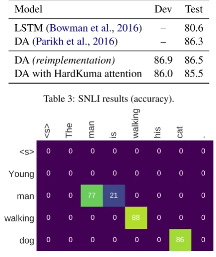
Results. With a target rate of 10%, the Hard-Kuma model achieved 8.5% non-zero attention. Table3shows that, even with so many zeros in the attention matrices, it only does about 1% worse compared to the DA baseline. Figure6shows an example of HardKuma attention, with additional examples in AppendixB. We leave further explo-rations with HardKuma attention for future work.
Model Dev Test
LSTM (Bowman et al.,2016) – 80.6
DA (Parikh et al.,2016) – 86.3
[image:7.595.75.283.255.369.2]DA(reimplementation) 86.9 86.5 DA with HardKuma attention 86.0 85.5
Table 3: SNLI results (accuracy).
<s>
The
man
is
walking
his
cat
.
<s>
Young
man
walking
dog
0 0 0 0 0 0 0 0
0 0 0 0 0 0 0 0
0 0 77 21 0 0 0 0
0 0 0 0 88 0 0 0
0 0 0 0 0 0 86 0
[image:7.595.306.525.468.728.2]7 Related Work
This work has connections with work on inter-pretability, learning from rationales, sparse struc-tures, and rectified distributions. We discuss each of those areas.
Interpretability. Machine learning research has been focusing more and more on interpretability (Gilpin et al., 2018). However, there are many nuances to interpretability (Lipton, 2016), and amongst them we focus on model transparency.
One strategy is to extract a simpler, inter-pretable model from a neural network, though this comes at the cost of performance. For example, Thrun (1995) extract if-then rules, while Craven and Shavlik(1996) extract decision trees.
There is also work on making word vectors more interpretable. Faruqui et al. (2015) make word vectors more sparse, andHerbelot and Vec-chi(2015) learn to map distributional word vectors to model-theoretic semantic vectors.
Similarly toLei et al.(2016),Titov and McDon-ald (2008) extract informative fragments of text by jointly training a classifier and a model pre-dicting a stochastic mask, while relying on Gibbs sampling to do so. Their focus is on using the sentiment labels as a weak supervision signal for opinion summarization rather than on rationaliz-ing classifier predictions.
There are also related approaches that aim to interpret an already-trained model, in contrast to Lei et al.(2016) and our approach where the ra-tionale is jointly modeled. Ribeiro et al. (2016) make any classifier interpretable by approximat-ing it locally with a linear proxy model in an approach called LIME, and Alvarez-Melis and Jaakkola(2017) propose a framework that returns input-output pairs that are causally related.
Learning from rationales. Our work is differ-ent from approaches that aim to improve clas-sification using rationales as an additional input (Zaidan et al., 2007; Zaidan and Eisner, 2008; Zhang et al.,2016). Instead, our rationales are la-tent and we are interested in uncovering them. We only use annotated rationales for evaluation.
Sparse layers. Also arguing for enhanced inter-pretability,Niculae and Blondel(2017) propose a framework for learning sparsely activated atten-tion layers based on smoothing the max opera-tor. They derive a number of relaxations tomax,
including softmax itself, but in particular, they target relaxations such as sparsemax (Martins and Astudillo, 2016) which, unlike softmax, are sparse (i.e. produce vectors of probability values with components that evaluate to exactly0). Their activation functions are themselves solutions to convex optimization problems, to which they pro-vide efficient forward and backward passes. The technique can be seen as a deterministic sparsely activated layer which they use as a drop-in replace-ment to standard attention mechanisms. In con-trast, in this paper we focus on binary outcomes rather thanK-valued ones. Niculae et al. (2018) extend the framework to structured discrete spaces where they learn sparse parameterizations of dis-crete latent models. In this context, parameter es-timation requires exact marginalization of discrete variables or gradient estimation via REINFORCE. They show that oftentimes distributions are sparse enough to enable exact marginal inference.
Peng et al. (2018) propose SPIGOT, a proxy gradient to the non-differentiable arg max op-erator. This proxy requires an arg max solver (e.g. Viterbi for structured prediction) and, like the straight-through estimator (Bengio et al.,2013), is a biased estimator. Though, unlike ST it is effi-cient for structured variables. In contrast, in this work we chose to focus on unbiased estimators.
Rectified Distributions. The idea of rectified distributions has been around for some time. The rectified Gaussian distribution (Socci et al.,1998), in particular, has found applications to factor anal-ysis (Harva and Kaban, 2005) and approximate inference in graphical models (Winn and Bishop, 2005).Louizos et al.(2017) propose to stretch and rectify samples from the BinaryConcrete (or Gum-belSoftmax) distribution (Maddison et al., 2017; Jang et al., 2017). They use rectified variables to induce sparsity in parameter space via a relax-ation toL0. We adapt their technique to promote
sparseactivations instead. Rolfe (2017) learns a relaxation of a discrete random variable based on a tractable mixture of a point mass at zero and a con-tinuous reparameterizable density, thus enabling reparameterized sampling from the half-closed in-terval[0,∞). In contrast, with HardKuma we fo-cused on giving support to both 0s and 1s.
8 Conclusions
for specifying how much text is to be extracted. To allow for reparameterized gradient estimates and support for binary outcomes we introduced the HardKuma distribution. Apart from extract-ing rationales, we showed that HardKuma has fur-ther potential uses, which we demonstrated on premise-hypothesis attention in SNLI. We leave further explorations for future work.
Acknowledgments
We thank Luca Falorsi for pointing us to Louizos et al. (2017), which inspired the Hard-Kumaraswamy distribution. This work has re-ceived funding from the European Research Coun-cil (ERC StG BroadSem 678254), the Euro-pean Union’s Horizon 2020 research and inno-vation programme (grant agreement No 825299, GoURMET), and the Dutch National Science Foundation (NWO VIDI 639.022.518, NWO VICI 277-89-002).
References
David Alvarez-Melis and Tommi Jaakkola. 2017. A causal framework for explaining the predictions of black-box sequence-to-sequence models. In Pro-ceedings of the 2017 Conference on Empirical Meth-ods in Natural Language Processing, pages 412– 421. Association for Computational Linguistics.
Yoshua Bengio, Nicholas L´eonard, and Aaron Courville. 2013. Estimating or propagating gradi-ents through stochastic neurons for conditional com-putation.arXiv preprint arXiv:1308.3432.
Samuel R. Bowman, Gabor Angeli, Christopher Potts, and Christopher D. Manning. 2015. A large anno-tated corpus for learning natural language inference. In Proceedings of the 2015 Conference on Empiri-cal Methods in Natural Language Processing, pages 632–642. Association for Computational Linguis-tics.
Samuel R. Bowman, Jon Gauthier, Abhinav Ras-togi, Raghav Gupta, Christopher D. Manning, and Christopher Potts. 2016. A fast unified model for parsing and sentence understanding. In Proceed-ings of the 54th Annual Meeting of the Association for Computational Linguistics (Volume 1: Long Pa-pers), pages 1466–1477. Association for Computa-tional Linguistics.
Qian Chen, Xiaodan Zhu, Zhen-Hua Ling, Si Wei, Hui Jiang, and Diana Inkpen. 2017. Enhanced lstm for natural language inference. InProceedings of the 55th Annual Meeting of the Association for Compu-tational Linguistics (Volume 1: Long Papers), pages 1657–1668. Association for Computational Linguis-tics.
Mark Craven and Jude W Shavlik. 1996. Extracting tree-structured representations of trained networks. In Advances in neural information processing sys-tems, pages 24–30.
Jacob Devlin, Ming-Wei Chang, Kenton Lee, and Kristina Toutanova. 2019. Bert: Pre-training of deep bidirectional transformers for language under-standing. InProceedings of the 2019 Conference of the North American Chapter of the Association for Computational Linguistics: Human Language Tech-nologies, Volume 1 (Long Papers). Association for Computational Linguistics.
Manaal Faruqui, Yulia Tsvetkov, Dani Yogatama, Chris Dyer, and Noah A. Smith. 2015. Sparse overcom-plete word vector representations. In Proceedings of the 53rd Annual Meeting of the Association for Computational Linguistics and the 7th International Joint Conference on Natural Language Processing (Volume 1: Long Papers), pages 1491–1500. Asso-ciation for Computational Linguistics.
Leilani H Gilpin, David Bau, Ben Z Yuan, Ayesha Ba-jwa, Michael Specter, and Lalana Kagal. 2018. Ex-plaining explanations: An overview of interpretabil-ity of machine learning. In 2018 IEEE 5th Inter-national Conference on Data Science and Advanced Analytics (DSAA), pages 80–89. IEEE.
Markus Harva and Ata Kaban. 2005. A variational bayesian method for rectified factor analysis. In
Proceedings. 2005 IEEE International Joint Confer-ence on Neural Networks, 2005., volume 1, pages 185–190. IEEE.
Aur´elie Herbelot and Eva Maria Vecchi. 2015. Build-ing a shared world: mappBuild-ing distributional to model-theoretic semantic spaces. In Proceedings of the 2015 Conference on Empirical Methods in Natural Language Processing, pages 22–32. Association for Computational Linguistics.
Sepp Hochreiter and J¨urgen Schmidhuber. 1997.
Long Short-Term Memory. Neural Computation, 9(8):1735–1780.
Jeremy Howard and Sebastian Ruder. 2018. Universal language model fine-tuning for text classification. In
Proceedings of the 56th Annual Meeting of the As-sociation for Computational Linguistics (Volume 1: Long Papers), pages 328–339. Association for Com-putational Linguistics.
Eric Jang, Shixiang Gu, and Ben Poole. 2017. Categor-ical reparameterization with gumbel-softmax. Inter-national Conference on Learning Representations.
MichaelI. Jordan, Zoubin Ghahramani, TommiS. Jaakkola, and LawrenceK. Saul. 1999. An intro-duction to variational methods for graphical models.
Machine Learning, 37(2):183–233.
Ponnambalam Kumaraswamy. 1980. A generalized probability density function for double-bounded random processes. Journal of Hydrology, 46(1-2):79–88.
Tao Lei, Regina Barzilay, and Tommi Jaakkola. 2016.
Rationalizing neural predictions. InProceedings of the 2016 Conference on Empirical Methods in Nat-ural Language Processing, pages 107–117. Associ-ation for ComputAssoci-ational Linguistics.
Zachary Chase Lipton. 2016. The mythos of model interpretability. ICML Workshop on Human Inter-pretability in Machine Learning (WHI 2016).
Christos Louizos, Max Welling, and Diederik P Kingma. 2017. Learning sparse neural net-works through l 0 regularization. arXiv preprint arXiv:1712.01312.
Chris J. Maddison, Andriy Mnih, and Yee Whye Teh. 2017. The concrete distribution: A continous re-laxation of discrete random variables. International Conference on Learning Representations.
Andre Martins and Ramon Astudillo. 2016. From soft-max to sparsesoft-max: A sparse model of attention and multi-label classification. In International Confer-ence on Machine Learning, pages 1614–1623.
Julian McAuley, Jure Leskovec, and Dan Jurafsky. 2012. Learning attitudes and attributes from multi-aspect reviews. InData Mining (ICDM), 2012 IEEE 12th International Conference on, pages 1020– 1025. IEEE.
Eric Nalisnick and Padhraic Smyth. 2016. Stick-breaking variational autoencoders. arXiv preprint arXiv:1605.06197.
Vlad Niculae and Mathieu Blondel. 2017. A regular-ized framework for sparse and structured neural at-tention. InAdvances in Neural Information Process-ing Systems, pages 3338–3348.
Vlad Niculae, Andr´e F. T. Martins, and Claire Cardie. 2018. Towards dynamic computation graphs via sparse latent structure. InProceedings of the 2018 Conference on Empirical Methods in Natural Lan-guage Processing, pages 905–911. Association for Computational Linguistics.
Ankur Parikh, Oscar T¨ackstr¨om, Dipanjan Das, and Jakob Uszkoreit. 2016. A decomposable attention model for natural language inference. In Proceed-ings of the 2016 Conference on Empirical Methods in Natural Language Processing, pages 2249–2255. Association for Computational Linguistics.
Hao Peng, Sam Thomson, and Noah A. Smith. 2018.
Backpropagating through structured argmax using a spigot. In Proceedings of the 56th Annual Meet-ing of the Association for Computational LMeet-inguistics (Volume 1: Long Papers), pages 1863–1873. Asso-ciation for Computational Linguistics.
Matthew Peters, Mark Neumann, Mohit Iyyer, Matt Gardner, Christopher Clark, Kenton Lee, and Luke Zettlemoyer. 2018. Deep contextualized word repre-sentations. InProceedings of the 2018 Conference of the North American Chapter of the Association for Computational Linguistics: Human Language Technologies, Volume 1 (Long Papers), pages 2227– 2237. Association for Computational Linguistics.
Danilo Jimenez Rezende, Shakir Mohamed, and Daan Wierstra. 2014. Stochastic backpropagation and ap-proximate inference in deep generative models. In
Proceedings of the 31st International Conference on Machine Learning, volume 32 ofProceedings of Machine Learning Research, pages 1278–1286, Be-jing, China. PMLR.
Marco Ribeiro, Sameer Singh, and Carlos Guestrin. 2016.“why should i trust you?”: Explaining the pre-dictions of any classifier. InProceedings of the 2016 Conference of the North American Chapter of the Association for Computational Linguistics: Demon-strations, pages 97–101. Association for Computa-tional Linguistics.
Jason Tyler Rolfe. 2017. Discrete variational autoen-coders. InICLR.
Nicholas D. Socci, Daniel D. Lee, and H. Sebastian Seung. 1998. The rectified gaussian distribution. In M. I. Jordan, M. J. Kearns, and S. A. Solla, editors,
Advances in Neural Information Processing Systems 10, pages 350–356. MIT Press.
Richard Socher, Alex Perelygin, Jean Wu, Jason Chuang, Christopher D. Manning, Andrew Ng, and Christopher Potts. 2013. Recursive deep models for semantic compositionality over a sentiment tree-bank. In Proceedings of the 2013 Conference on Empirical Methods in Natural Language Process-ing, pages 1631–1642. Association for Computa-tional Linguistics.
Sebastian Thrun. 1995. Extracting rules from artificial neural networks with distributed representations. In
Advances in neural information processing systems, pages 505–512.
Ivan Titov and Ryan McDonald. 2008. A joint model of text and aspect ratings for sentiment summariza-tion. InProceedings of ACL.
Ronald J Williams. 1992. Simple statistical gradient-following algorithms for connectionist reinforce-ment learning. Machine learning, 8(3-4):229–256.
John Winn and Christopher M Bishop. 2005. Varia-tional message passing. Journal of Machine Learn-ing Research, 6(Apr):661–694.
Omar Zaidan, Jason Eisner, and Christine Piatko. 2007.
Using “annotator rationales” to improve machine learning for text categorization. In Human Lan-guage Technologies 2007: The Conference of the North American Chapter of the Association for Computational Linguistics; Proceedings of the Main Conference, pages 260–267. Association for Com-putational Linguistics.
Ye Zhang, Iain Marshall, and Byron C. Wallace. 2016.
A Kumaraswamy distribution
0.0 0.2 0.4 0.6 0.8 1.0 0.0
0.5 1.0 1.5 2.0 2.5
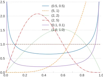
[image:12.595.78.283.102.256.2](0.5, 0.5) (5, 1) (2, 2) (2, 5) (0.1, 0.1) (1.0, 1.0)
Figure 7: Kuma plots for various (a, b) parameters.
A Kumaraswamy-distributed variable K ∼
Kuma(a, b) takes on values in the open interval
(0,1)and has density
fK(k;a, b) =abka−1(1−ka)b−1, (17)
where a ∈ R>0 and b ∈ R>0 are shape
param-eters. Its cumulative distribution takes a simple closed-form expression
FK(k;a, b) =
Z k
0
fK(ξ|a, b)dξ (18a)
= 1−(1−ka)b , (18b)
with inverse
FK−1(u;a, b) =
1−(1−u)1/b 1/a
. (19)
A.1 Generalised-support Kumaraswamy
We can generalise the support of a Kumaraswamy variable by specifying two constants l < r and transforming a random variableK ∼Kuma(a, b)
to obtain T ∼ Kuma(a, b, l, r) as shown in (20, left).
t=l+ (r−l)k k=(t−l)/(r−l) (20)
The density of the resulting variable is
fT(t;a, b, l, r) (21a)
=fK
t−l
r−l;a, b
dk
dt
(21b)
=fK
t−l
r−l;a, b
1
(r−l) (21c)
wherer−l > 0by definition. This affine trans-formation leaves the cdf unchanged, i.e.
FT(t0;a, b, l, r) = Z t0
−∞
fT(t;a, b, l, r)dt
=
Z t0
−∞ fK
t−l
r−l;a, b
1
(r−l)dt
=
Z t0−l
r−l
−∞
fK(k;a, b) 1
(r−l)(r−l)dk =FK
t0−l
r−l;a, b
.
(22)
Thus we can obtain samples from this generalised-support Kumaraswamy by sampling from a uni-form distribution U(0,1), applying the inverse transform (19), then shifting and scaling the sam-ple according to (20, left).
A.2 Rectified Kumaraswamy
First, we stretch a Kumaraswamy distribution to include0and1in its support, that is, withl < 0
andr >1, we defineT ∼Kuma(a, b, l, r). Then we apply a hard-sigmoid transformation to this variable, that is, h = min(0,max(1, t)), which results in arectified distribution which gives sup-port to the closed interval [0,1]. We denote this rectified variable by
H∼HardKuma(a, b, l, r) (23) whose distribution function is
fH(h;a, b, l, r) =
P(h= 0)δ(h) +P(h= 1)δ(h−1)
+P(0< h <1)
fT(h;a, b, l, r)1(0,1)(h) P(0< h <1)
(24)
where
P(h= 0) =P(t≤0)
=FT(0;a, b, l, r) =FK(−l/(r−l);a, b) (25)
is the probability of sampling exactly0, where
P(h= 1) =P(t≥1) = 1−P(t <1)
= 1−FT(1;a, b, l, r) = 1−FK((1−l)/(r−l);a, b)
(26)
is the probability of sampling exactly 1, and
P(0< h <1) = 1−P(h= 0)−P(h= 1) (27)
A.3 Reparameterized gradients
Let us consider the case where we need deriva-tives of a functionL(u)of the underlying uniform variable u, as when we compute reparameterized gradients in variational inference. Note that
∂L ∂u =
∂L ∂h ×
∂h ∂t ×
∂t ∂k ×
∂k
∂u , (28)
by chain rule. The term ∂∂hLdepends on a differen-tiable observation model and poses no challenge; the term ∂h∂t is the derivative of the hard-sigmoid function, which is 0 for t < 0 or t > 1, 1 for
0 < t < 1, and undefined for t ∈ {0,1}; the term ∂k∂t = r−lfollows directly from (20, left); the term ∂k∂u = ∂u∂ FK−1(u;a, b) depends on the Kumaraswamy inverse cdf (19) and also poses no challenge. Thus the only two discontinuities hap-pen fort∈ {0,1}, which is a0measure set under the stretched Kumaraswamy: we say this reparam-eterisation is differentiable almost everywhere, a useful property which essentially circumvents the discontinuity points of the rectifier.
A.4 HardKumaraswamy PDF and CDF
Figure8 plots the pdf of the HardKumaraswamy for various a and b parameters. Figure9does the same but with the cdf.
Figure 8: HardKuma pdf for various (a, b).
B Implementation Details
B.1 Multi-aspect Sentiment Analysis
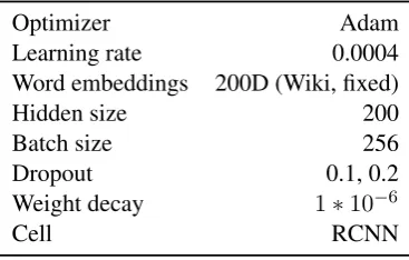
[image:13.595.311.522.67.228.2]Our hyperparameters are taken from Lei et al. (2016) and listed in Table 4. The pre-trained word embeddings and data sets are available on-line at http://people.csail.mit.edu/ taolei/beer/. We train for 100 epochs and
Figure 9: HardKuma cdf for various (a, b).
select the best models based on validation loss. For the MSE trade-off experiments on all aspects combined, we train for a maximum of 50 epochs.
Optimizer Adam
Learning rate 0.0004 Word embeddings 200D (Wiki, fixed)
Hidden size 200
Batch size 256
Dropout 0.1, 0.2
Weight decay 1∗10−6
[image:13.595.324.508.348.465.2]Cell RCNN
Table 4: Beer hyperparameters.
For the Bernoulli baselines we varyL0 weight
λ1 among{0.0002,0.0003,0.0004}, just as in the
original paper. We set the fused lasso (coherence) weightλ2to2∗λ1.
For the HardKuma models we set a target se-lection rate to the values targeted in Table2, and optimize to this end using the Lagrange multi-plier. We chose the fused lasso weight from {0.0001,0.0002,0.0003,0.0004}.
B.1.1 Recurrent Unit
[image:13.595.77.288.454.610.2]Lei et al.(2016), which is defined as: λt=σ(Wλxt+Uλht−1+bλ) c(1)t =λtc(1)t−1+ (1−λt)W1xt
c(2)t =λtct(2)−1+ (1−λt)(c (1)
t−1+W2xt)
ht= tanh
c(2)t +b
B.1.2 Expected values for dependent latent variables
The expectedL0is a chain of nested expectations,
and we solve each term
Ep(zi|x,z<i)[I[zi 6= 0]|z<i]
= 1−FK
−l
r−l;ai, bi
(29)
as a function of a sampled prefix, and the shape parametersai, bi = gi(x, z<i;φ)are predicted in
sequence.
B.2 Sentiment Classification (SST)
For sentiment classification we make use of the PyTorch bidirectional LSTM module for encod-ing sentences, for both the rationale extractor and the classifier. The BiLSTM final states are con-catenated, after which a linear layer followed by a softmax produces the prediction. Hyperparame-ters are listed in Table5. We apply dropout to the embeddings and to the input of the output layer.
Optimizer Adam
Learning rate 0.0002
Word embeddings 300D Glove (fixed)
Hidden size 150
Batch size 25
Dropout 0.5
Weight decay 1∗10−6
Cell LSTM
Table 5: SST hyperparameters.
B.3 Natural Language Inference (SNLI)
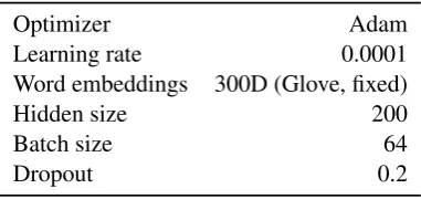
Our hyperparameters are taken fromParikh et al. (2016) and listed in Table6. Different fromParikh et al. is that we use Adam as the optimizer and a batch size of 64. Word embeddings are projected to 200 dimensions with a trained linear layer. Un-known words are mapped to 100 unUn-known word classes based on the MD5 hash function, just as inParikh et al.(2016), and unknown word vectors are randomly initialized. We train for 100 epochs,
evaluate every 1000 updates, and select the best model based on validation loss. Figure10 shows a correct and incorrect example with HardKuma attention for each relation type (entailment, con-tradiction, neutral).
Optimizer Adam
Learning rate 0.0001
Word embeddings 300D (Glove, fixed)
Hidden size 200
Batch size 64
[image:14.595.321.512.141.231.2]Dropout 0.2
<s>
The
two
dogs
are
black
.
<s>
Two
black
dogs
running
0 0 0 0 0 0 0
0 0 0 0 0 0 0
0 0 0 0 0 100 0
0 0 0 90 0 0 0
0 0 0 23 0 0 0
(a) Entailment (correct)
<s> Four people in a kitchen cooking .
<s> Four people in a kitchen
0 0 0 0 0 0 0 0
0 89 0 0 0 0 0 0
0 0 53 0 0 0 0 0
0 0 0 0 0 0 0 0
0 0 0 0 0 0 0 0
0 0 0 0 0 100 74 0
(b) Entailment (incorrect, pred: neutral)
<s> Three cats race on a track .
<s> Three dogs racing on racetrack
0 0 0 0 0 0 0 0
0 84 0 0 0 0 0 0
0 0 100 0 0 0 18 0
0 0 0 87 0 0 43 0
0 0 0 0 0 0 0 0
0 0 33 48 0 0 73 0
(c) Contradiction (correct)
<s>
a
couple
on
a
motorcycle
<s>
A
person
on
a
motorcycle
.
0 0 0 0 0 0
0 0 0 0 0 0
0 0 15 0 0 0
0 0 0 0 0 0
0 0 0 0 0 0
0 0 0 0 0 89
0 0 0 0 0 0
(d) Contradiction (incorrect, pred: entailment)
<s>
They
are
in
the
desert
.
<s>
People
walking
through
dirt
.
0 0 0 0 0 0 0
0 0 0 0 0 0 0
0 0 0 0 0 0 0
0 0 0 0 0 0 0
0 0 0 0 0 81 0
0 0 0 0 0 0 0
(e) Neutral (correct)
<s> A dog found a bone
<s> A
dog
gnawing
on
a bone
.
0 0 0 0 0 0
0 0 0 0 0 0
0 0 89 13 0 12
0 0 0 0 0 47
0 0 0 0 0 0
0 0 0 0 0 0
0 0 12 14 0 76
0 0 0 0 0 0
[image:15.595.96.507.81.721.2](f) Neutral (incorrect, pred: entailment)