Hyperspectral texture analysis for colon tissue biopsy classification

http://wrap.warwick.ac.uk/

Original citation:

Masood, Khalid, Rajpoot, Nasir M. (Nasir Mahmood), Qureshi, Hammad A. and Rajpoot,

K. (2007) Hyperspectral texture analysis for colon tissue biopsy classification. In:

International Symposium on Health Informatics and Bioinformatics (HIBIT 2007),

Antalya, Turkey, 30 April - May 2 2007

Permanent WRAP url:

http://wrap.warwick.ac.uk/61636

Copyright and reuse:

The Warwick Research Archive Portal (WRAP) makes this work by researchers of the

University of Warwick available open access under the following conditions. Copyright ©

and all moral rights to the version of the paper presented here belong to the individual

author(s) and/or other copyright owners. To the extent reasonable and practicable the

material made available in WRAP has been checked for eligibility before being made

available.

Copies of full items can be used for personal research or study, educational, or

not-for-profit purposes without prior permission or charge. Provided that the authors, title and

full bibliographic details are credited, a hyperlink and/or URL is given for the original

metadata page and the content is not changed in any way.

A note on versions:

The version presented in WRAP is the published version or, version of record, and may

be cited as it appears here.For more information, please contact the WRAP Team at:

HYPERSPECTRAL TEXTURE ANALYSIS FOR COLON TISSUE BIOPSY

CLASSIFICATION

Khalid Masood, Nasir Rajpoot, Hammad Qureshi

Department of Computer Science

University of Warwick

Coventry, CV4 7AL, UK

Kashif Rajpoot

Wolfson Medical Vision Lab

University of Oxford

UK

ABSTRACT

Diagnosis and cure of colon cancer can be improved by performing automated histopathological analysis of colon biopsy samples. Due to significant observational variation between pathologists in several histological features, there is a need for the development of automated, quantitative analysis techniques. This paper presents a promising au-tomative technique for the classification of hyperspectral colon tissue biopsy images. The application of hyperspec-tral imaging techniques in medical image analysis is a new domain for researchers. The main advantage of using hy-perspectral imaging is the increased spectral resolution and detailed subpixel information. The proposed classification algorithm is based on the subspace projection techniques particularly Support Vector Machines (SVM) with Gaus-sian Kernel. Dimensionality reduction and tissue segmenta-tion is achieved by Independent Component Analysis (ICA) andk-means clustering. Morphological features, which de-scribe the shape, orientation and other geometrical attributes, are extracted in first set of experiments. Grey level co-occurrence matrices are computed for the second set of ex-periments. The SVM with appropriate choice of parame-ters for its Gaussian kernel efficiently exploits the non linear boundary between the benign and malignant classes of the colon tissue biopsies.

1. INTRODUCTION

Colon cancer is a malignant disease of the large bowel. Af-ter lung and breast cancer, colorectal cancer (a combined term for colon and rectal cancer) is the most common cause of death for cancers in the Western world. The incidence of disease in England and Wales is about 30,000 cases/year, resulting in approximately 17,000 death/annum [13], and it has been estimated that at least half a million cases of col-orectal cancer occur each year worldwide. It is caused by colonic polyps, an abnormal growth of tissue that projects in due course from the lining of the intestine or rectum, into colorectal cancer. These polyps are often benign and usually

produce no symptoms. They may, however, cause painless rectal bleeding usually not apparent to the naked eye. The normal time for a polyp to reach 1 cm in diameter is five years or a little more. This 1 cm polyp will take around 5-10 years for the cancer to cause symptoms by which time it is frequently too late [11].

Diets low in fruits, less protein from vegetable sources, high age and family history are associated with increased risk of polyps. Persons smoking more than 20 cigarettes a day are 250 percent more likely to have polyps as opposed to nonsmokers who otherwise have the same risks. There is an association of cancer risk with meat, fat or protein con-sumption which appear to break down in the gut into cancer causing compounds called carcinogens [8]. Smoking ces-sation is important to decrease the likelihood of developing colon cancer. Dietary supplementation with 1500 mg of cal-cium or more a day is associated with a lower incidence of colon cancer. Weight reduction may be helpful in reducing the risk for colorectal cancer. Daily exercise reduces the likelihood of developing colon cancer. Turmeric, the spice which gives curry its distinctive yellow color, may also pre-vent colon cancer [5].

1.1. Hyperspectral Imaging

Hyperspectral imaging in laboratory experiments, is a non-contact sensing technique for obtaining both spectral and spatial information about a tissue sample. Hyperspectral imaging measures a spectrum for each pixel in an image. There are many types of spectroscopy which are being used to study the spectral signatures of individual cells and un-derlying tissue sections. In optical spectroscopy, which mea-sures transmission through, or reflectance from, a sample by visible or near-infrared radiation at the same wavelength as the source, classification is done mostly by statistical mea-sures [1].

Spectrometers are used to make measurements of the light reflected from a test specimen. A prism in the centre of spectrometer splits this light into many different wavelength bands and the energy in each band is measured by detectors which are different for each band. By using large number of detectors (even a few thousand), spectrometers can make spectral measurements of bands as narrow as 0.01 microm-eters over a wide wavelength range, typically at least 0.4 to 2.4 micrometers (visible through middle infrared wave-length ranges). Most approaches to analyse hyperspectral images concentrate on the spectral information in ual image cells, rather than spatial variations within individ-ual bands or groups of bands. The statistical classification (clustering) methods often used with multispectral images can also be applied to hyperspectral images but may need to be adapted to handle high dimensionality.

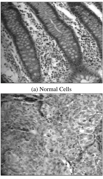
Recent developments in hyperspectral imaging have en-hanced the usefulness of the light microscope [3]. A stan-dard epifluorescence microscope can be optically coupled to an imaging spectrograph, with output recorded by a CCD camera. Individual images are captured representing Y-wave-length planes, with the stage successively moved in the X di-rection, allowing an image cube to be constructed from the compilation of generated scan files. Hyperspectral imaging microscopy permits the capture and identification of differ-ent spectral signatures presdiffer-ent in an optical field during a single-pass evaluation, including molecules with overlap-ping but distinct emission spectra. High resolution charac-teristics of hyperspectal imaging is reflected in two sample images in Figure 1 of colon tissue cells.

1.2. Related Work

A computational model of light interaction with colon tis-sue and classification using the tistis-sue reflectance spectra is analyzed in [16]. Three layers: mucosa, submucosa and smooth muscle, have different reflectance properties with the light incident on their surface. Different parameters characterising the mucosa layer include blood volume frac-tion, haemoglobin saturafrac-tion, the size of the collagen fibres, their density and the layer thickness, have unique changes for the emitted spectra of normal and malignant colon tis-sues. Fifty normal and seven cancerous tissues were used as an input to the system. Thus it is claimed that above model correctly predicts the spectra of colon tissue and this is in agreement with known histological changes which occur with the development of cancer which alters the macroar-chitecture of the colon tissue.

Mass spectrometry, classification of samples using dif-ference in their molecular weights, is used in [10] for the probabilistic classification of healthy vs. disease whole serum samples. The approach employs PCA followed by LDA on mass spectrometry data of complex protein mixtures. Clas-sification is done on the principle that healthy spectrum lies

(a) Normal Cells

(b) Malignant Cells

Fig. 1. Colon Tissue Imagery

closer to the healthy cluster than to the disease cluster (and vice-versa). Test spectra can than be classified by minimum distance to its nearest cluster. Linear discriminant analysis creates a hyperplane that maximises the between-class vari-ance while minimising the within-class varivari-ance.

2. DIMENSIONALITY REDUCTION AND SUBSPACE PROJECTION

2.1. Independent Component Analysis (ICA)

The objective of Independent Component Analysis (ICA) is to perform a dimension reduction approach to achieve decorrelation between independent components [18]. Let us denote byX = (x1, x2, . . . , xm)

T

a zero-mean m-dimensional variable, andS = (s1, s2, . . . , sn)

T

,n < m, is its linear transform with a constant matrixW [17]:

S=W X

Given X as observations, ICA aims to estimating W and S. The goal of ICA is to find a new variable S such that trans-formed componentssiare not only uncorrelated with each

other, but also statistically as independent of each other as possible. An ICA algorithm consists of two parts, an ob-jective function which measures the independence between components, entropy of each independent source or their higher order cumulants, and the second part is the optimisa-tion method used to optimise the objective funcoptimisa-tion. Higher order cumulants like kurtosis, and approximations of ne-gentropy provide one-unit objective function. A decorrela-tion method is needed to prevent the objective funcdecorrela-tion from converging to the same optimum for different independent components. Whitening or data sphering project the data onto its subspace as well as normalizing its variance.

2.2. K-Means Clustering

Clustering is the process of partitioning or grouping a given set of patterns into disjoint clusters. This is done such that patterns in the same cluster are alike and patterns belonging to two different clusters are different. Thek-means method has been shown to be effective in producing good clustering results for many practical applications [2]. The aim of thek -means algorithm is to dividempoints inndimensions into

kclusters so that the within-cluster sum of squared distance from the cluster centroids is minimised. The algorithm re-quires as input a matrix ofmpoints in ndimensions and a matrix ofk initial cluster centres inndimensions. The number of clusterskis assumed to be fixed ink-means clus-tering. Let thekprototypes(w1, . . . , wk)be initialised to one of theminput patterns(i1, . . . , im). Therefore;

wj =il, j∈ {1, . . . , k}, l∈ {1, . . . , m}

The appropriate choice ofkis problem and domain depen-dent and generally a user must try several values ofk. The quality of the clustering is determined by the following error function:

E =

k

X

j=1

X

il∈Cj

|il−wj|2

The direct implementation ofk-means method is computa-tionally very intensive.

2.3. Support Vector Machine (SVM)

Support vector machine (SVM) introduces a nonlinear map-ping from the input space to an implicit high-dimensional feature space, where the nonlinear and complex distribu-tions of the patterns in the input space is linearized so that a linear separating boundary can be applied for the classi-fication [14]. Suppose that data is mapped to some other (possibly infinite dimensional) euclidean spaceH using a mapping functionφ:

φ:Rd−→Hn

The mapping algorithm depend on the data through dot products in H in the form ofφ(xi).φ(xj). Now if there is

a kernel functionKwhich can do the required dot products than there is no need of finding the dot product themselves. This ia called the kernel trick. Kernel functionKshould be such that;

K(xi, xj) =φ(xi).φ(xj)

AsHis possibly infinite dimesional andnis much higher thand, so a linear separation is more straightforward. The introduction of the kernel function provides the allowance to avoid the explicit evaluation of mapping. There are sev-eral kernel functions available but polynomial, gaussian and sigmoidal kernel are used mor often. The choice of kernel depends on the data and its clusterring. Gaussian kernel is used in most cases because of its parameter selection [15]. It is defined as;

K(xi, xj) =e−γ(xi−xj)2_+C

There is one common parameterCwhich is called con-stant of constraint. It is defined as the clusterring of the data on the wrong side of the margin. It is constant for each data and it does not affect the tuning of the kernel. The other parameter for Gaussian kernel is the width of gaussian basis functionγ. Its selection depends on the input data and vari-ety of selection methods are used including grid search and newton bisection methods. Once a kernel is tuned properly, classification of test data is performed very accurately.

3. METHODOLOGY

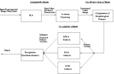
The proposed classification algorithm consists of three mod-ules as shown in Figure 2. Brief description of dimensional-ity reduction and feature extraction modules is given in the following sub-sections. Detailed description of the segmen-tation can be found in [14].

3.1. Segmentation

Fig. 2. Classification Algorithm Block Diagram

data has to be dimensionally reduced. Dimensionality re-duction involves two steps, extraction of statistically inde-pendent components using Indeinde-pendent Component Anal-ysis (ICA) and colour segmentation usingk-means cluster-ing. Flexible ICA (FlexICA) [6], a fixed point algorithm for ICA, adopting a generalised Gaussian density, is used for data sphering (whitening) and achieves considerable di-mensionality reduction. Data is distributed towards heavy-tailedness by the high-emphasis filters. The data with re-duced dimensionality is then fed tok-means clustering al-gorithm for segmentation.

The hyperspectal data cube containing 128 subbands is segmented into four labeled parts. Each slide of the tissue cells is divided into four regions represented by four colours as shown in Figure 3. The four labeled parts are denoted by colours as dark blue for nuclei, light blue for cytoplasm, yellow for gland secretions and red for lamina propria.

3.2. Feature Extraction

3.2.1. Morphological Features

In order for the pattern recognition process to be tractable it is necessary to represent patterns into some mathematical or analytical model. The model should convert patterns into features or measurable values, which are condensed repre-sentations of the patterns, containing only salient informa-tion [7]. Morphological features, which describe the shape, size, orientation and other geometrical attributes of the cel-lular components, are extracted to discriminate between two classes of input data. The segmented image is first split into four binarised image in accordance with the four cellular components. In each binary image, the corresponding cel-lular components i.e. nuclei, cytoplasm, gland secretions and stroma of lamina propria have binary value equal to 1.

(a) Benign Cells

(b) Malignant Cells

Fig. 3. Segmentation Results

3.2.2. Co-occurnence Features

The co-coourrence approach is based on the grey level spa-tial dependence. Co-occurrence matrix is computed by second-order joint conditional probability density functionf(i, j|d, θ). Eachf(i, j|d, θ)is computed by counting all pairs of pixels separated by distancedhaving grey levelsiandj, in the given directionθ. The angular displacementθusually takes on the range of values from θ = 0,45,90,135 degrees. The co-occurrence matrix captures a significant amount of textural information. The diagonal values for a coarse tex-ture are high while for a fine textex-ture these diagonal values are scattered. To obtain rotataion invariant features the co-occurrence matrices obtained from the different directions are accumulated. The three set of attributes used in our ex-periments are Energy, Inertia and Local Homogeneity.

E=X

i

X

j

[f(i, j|d, θ)]2

I=X

i

X

j

[(i−j)2f(i, j|d, θ)]

LH=X

i

X

j

4. EXPERIMENTS

4.1. Experimental Setup

The experimental setup consists of a CRI Nuance micro-scope and a CCD camera. Two different datasets are pre-pared. Each dataset contains ten biopsy images of the colon biopsies on a tissue micro-array. These samples come from different patients and are prepared byH&Estaining. Each slide is illuminated with a tuned light source (capable of emitting any combination of light frequencies in the range of 450-850 nm), followed by magnification to 400 X. Thus several images, each image using a different combination of light frequencies, are produced [4]. Dataset I contains ten biopsy slides with 32 hyperspectral bands and each slide has a 1024x1024 resolution. 128 hyperspectral bands are used in dataset II with 491x652 resolution for each band.

The first set of experiments is carried out with morpho-logical feature extraction method. Each image is divided into64×64blocks or patches. Morphological operation is performed on the patches for extraction of feature vec-tors using different combinations of ten scalar morpholog-ical properties. The testing is done on the format of leave one out (LOO) and blocks from nine slides make training set while blocks from the tenth slide is used for testing. Eu-ler number, area, extent, convex area, equivalent diameter and other elliptical parameters are calculated for each block. Using ten parameters for each binary image, a feature vector containing 40 dimensions represents each block. PCA with twenty principal components is employed in the first exper-iment. Supervision in the training set is introduced through LDA in the second experiment. Third experiment uses SVM with gaussian kernel. Its tunning is done with newton bisec-tion method which gives it sufficient bandwidth to achieve a resonable classification accuracy.

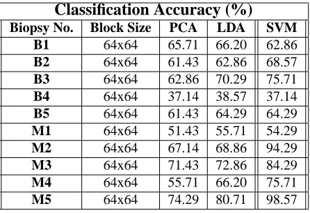
4.2. Experiments with Co-occurrence Features

The second set of experiments uses directional textural at-tributes which are extracted for each block. Dataset II is used becuase it has less resolution as compared to dataset I. Co-occurrence matrix is computed for the block size of 64x64 for each slide. Three co-occurrence features, con-taining angular second moment (Energy), variance and ho-mogenity, are calculated while pixel distance is varied from one pixel to two pixel values. Four directional features in the direction of 0, 45, 90 and 135 are concatanated together so that a feature vector with 24 dimensions is used in the classifiers. PCA nd LDA are used in first two experiments. The last experiment is carried out with SVMs. Gaussian kernel with grid search tunning method is used with con-stant of constraint having very small value.

4.3. Results

Classification Accuracy (%)

B1 64x64 64.55 68.57 68.57 B2 64x64 53.66 56.76 78.57 B3 64x64 55.88 54.36 75.71 B4 64x64 53.64 54.36 77.14 B5 64x64 57.93 59.64 64.29 M1 64x64 41.55 45.22 75.71 M2 64x64 47.75 49.26 62.86 M3 64x64 61.91 61.95 74.29 M4 64x64 51.54 52.63 75.71 M5 64x64 53.54 55.29 78.57

Table 1. Morphological Features

The classification accuracy in the morphological set of experiments is about 80 percent with PCA and LDA. Eight slides on the whole are classified correctly with a threshold of 50 percent on the patches. SVM gives an accuracy of 90 percent with 9 slides out of ten are being classified in the true classes. With directional textural features, blocks clas-sification accuracy increases for each slide in comparison to first set of experiments. Overall slide accuracy is upto 90 percent. SVM again outperforms PCA and LDA. One way of explanation can be such that SVM introduces a nonlin-ear mapping from the input space which make classification of nonlinear boundary patterns similar to linear boundary problems.

5. CONCLUSIONS

In this paper, classification of colon tissue cells is achieved using the morphology of the glandular cells of the tissue

re-Classification Accuracy (%)

B1 64x64 65.71 66.20 62.86 B2 64x64 61.43 62.86 68.57 B3 64x64 62.86 70.29 75.71 B4 64x64 37.14 38.57 37.14 B5 64x64 61.43 64.29 64.29 M1 64x64 51.43 55.71 54.29 M2 64x64 67.14 68.86 94.29 M3 64x64 71.43 72.86 84.29 M4 64x64 55.71 66.20 75.71 M5 64x64 74.29 80.71 98.57

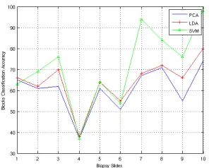
Co-occurrence Features Classification

Fig. 4. Blocks Classification Accuracy

gion. There is an indication that the morphology of the cells, obtained from the hyperspectral analysis of biopsy slides, has strong discriminatory power. Regular structured cell shapes with fine orientation of the tissue glands are char-acteristics of normal cells, whereas irregular and deformed glandular shapes represent malignant tissue. In morpholog-ical analysis, five features’ subset achieves accuracy upto 90 percent on whole biopsy images. In the second set of ex-periments with gray level co-occurrence matrix and using a feature vector of 24 dimensions, reasonable classification is performed even with simple classifiers like LDA. However, employing properly tuned Gaussian kernel with grid search method, accuracy, even for individual blocks, is quite good.

6. REFERENCES

[1] John Adams, M. Smith, and A. Gillespie. Imaging spectroscopy: Interpretation based on specral mixture analysis. Remote Geochemical Analysis, 1993.

[2] K. Alsabti, S. Ranka, and V. Singh. An efficient k-means clustering algorithm. www.cise.ufl.edu., 1997.

[3] E. A. Cloutis. Hyperspectral geological remote sensing. Evaluation of Analytical Techniques-International Journal of Remote Sensing, 17:2215–

2242, 1996.

[4] G. Davis, M. Maggioni, and R. Coifman et al. Spec-tral/spatial analysis of colon carcinoma. Journal of

Modern Pathology, 2003.

[5] R. S. Houlston. Molecular pathology of of colorectal cancer. Clinical Pathology, 2001.

[6] A. Hyvarinen. Survey on independent component analysis. Neural Computing Surveys, 2:94–128, 1999.

[7] Anil Jain, Robert Duin, and Jianchang Mao. Statistical pattern recognition: A review. IEEE Trans. on Pattern

Analysis and Machine Intelligence, 22, 2000.

[8] S. Kaster, S. Buckley, and T. Haseman. Colonoscopy and barium enema in the detection of colorectal can-cer. Gastrointestinal Endoscopy, 1995.

[9] David Landgrebe. Hyperspectral image data analy-sis as a high dimensional signal processing problem.

IEEE Signal Processing magazine, 2002.

[10] Ryan Lilien, Hany Farid, and Bruce Donald. Proba-bilistic disease classification of expression-dependent proteomic data from mass spectrometry of human serum. Journal of Computational Biology, 2003.

[11] D. E. Mansell. Colon polyps & colon cancer.

Amer-ican Cancer Society Textbook of Clinical Oncology,

1991.

[12] T. Mattfeldt, H. Gottfried, and V. Schmidt. Classi-fication of spatial textures in benign and cancerous glandular tissues by stereology and stochastic geom-etry using artificial neural networks. Journal of

Mi-croscopy, 2000.

[13] Office of National Statistics. Cancer statistics: Regis-trations, england and wales. london. HMSO, 1999.

[14] K. M. Rajpoot and Nasir M Rajpoot. Hyperspectral colon tissue cell classification. SPIE Medical Imaging

(MI), 2004.

[15] N. Rajpoot and K. Masood. Human gait recognition with 3-d wavelets & kernel based subspace projec-tions. International Workshop on HAREM, 2005.

[16] Dzena Rowe, Ela Claridge, and Tariq Ismail. Analysis of multispectral images of the colon to reveal histolog-ical changes characteristic of cancer. MIUA, 2006.

[17] Chen-Hsiang Yeang, Sridhar Ramaswamy, and Pablo Tamayo et al. Molecular classification of multi-ple tumor types. Bioinformatics, 2001.

[18] Kun Zhang and Lai-Wan Chan. Dimension reduction based on orthogonality-a decorrelation method in ica.