Preface
Trailing Suction Hopper Dredgers (TSHD), are self-propelled vessels which contain
large tanks for transferring sand or slurry. Dredging installations are used on board
of these vessels to load and unload the sand. TSHDs work in consecutive cycles
with four phases: 1. sailing empty to the loading area, 2. filling the hopper, 3. sailing
full to the discharge area, 4. unloading the material.
The aim of this study was to develop a method to reduce propeller thrust and
consequently fuel consumption during the two sailing phases of TSHDs.
The task was done by developing a novel control method for automatic
steer-ing of TSHDs subject to various disturbances and limitations. The solution involved
trajectory planning, speed assignment and steering control which is applicable for
underactuated ships. The results of simulation experiments manifested accurate
trajectory tracking and reduced thrust. The reduced thrust implies reduced fuel
con-sumption; this benefit is mostly due to the fact that the novel control method allows
for a better distribution of required speeds.
This M.Sc. assignment was defined as a collaborative project between IMOTEC
B. V. and University of Twente.
The thesis is reported as two papers which are written in IEEE format. The
first paper entitled “Towards Automatic Steering of Underactuated Ships” has richer
scientific and technical content and is ready for publication. “Reducing Fuel
Con-sumption for Trailing Suction Hopper Dredgers” is an application paper where the
automatic steering control developed in first paper is employed to answer the
re-search question of this M.Sc. assignment.
Towards Automatic Steering of Underactuated Ships
Hengameh Noshahri
Abstract—Simple control solutions for steering underactuated ships have been seldom studied in literature. This paper provides a control method for automatic steering of underactuated ships in presence of disturbances and in uncertain environmental conditions. A mathematical model of ship dynamics is developed and validated. Our control method involves introduction of a preparation phase consisting of three algorithms. Waypoints leading to every desired set-point are defined and a continuous Dubins path is generated between these waypoints. A second-order motion profile is assigned to the path to suggest the speed with the best timing for the voyage. The control objective is reformulated from a tracking problem to a regulating problem by changing coordinates of the reference signal. PD-controllers are employed in closed loop to reduce position and heading error. The controller parameters are set in the design phase and do not need additional tuning for different trajectories and ship param-eters. Weather information together with the planned motion profile are used in a feedforward controller design to achieve better disturbance rejection and higher accuracy. Performance and robustness of the design are evaluated in simulation by Course-keeping and Course-changing experiments in extreme and uncertain environmental conditions. While the developed control method is simple compared to the methods in literature, it can still achieve quite satisfactory steering performance.
Keywords—Automatic steering, Control design, Mathematical model, Trajectory planning
I. INTRODUCTION
Commanding the rudder, propulsion system, and any other device on board of the ship to reach a specified position, is known as ship steering control. Automatic steering systems have been developed over the course of time to satisfy vari-ous purposes. A comprehensive overview of marine vessel’s control systems is provided in [1]. The concept of automatic ship control dates back to the 19th century and it was first
realized by fully mechanical autopilot designs. Later, by devel-opment of control theory and electronics, closed-loop control systems such as PID-controllers were introduced to correct the rudder angle. Problems associated with tuning of these controllers have led to using methods like pole placement, Linear Quadratic (LQ), Fuzzy, and Genetic Algorithms [2].
In a model-based ship-control approach, it is customary to consider a simplified version of ship dynamics. Single-Input-Single-Output (SISO) transfer function models, such as the Nomoto model [3], facilitate the use of linear control methods. These techniques can only command one variable, which is usually the rudder angle, to control the ship heading. Increased functionality of ship maneuvering however, requires more sophisticated control.
Non-linear Multi-Input-Multi-Output (MIMO) control meth-ods provide high performance features, but they need full measurements or observer systems to operate. State feedback
linearization, sliding mode, backstepping, and Lyapunovs di-rect control are among these methods. A survey on non-linear ship control can be found in [4]. These methods can gener-ally be characterized as complex; the underlying mathematics require a significant amount of skills and expertise.
A system is called fully actuated if it has one or more control inputs for each Degree of Freedom (DOF). A fully actuated ship with three-dimensional configuration space comprised of forward, sideways, and heading would require actuators capable of exerting forces and moments independently to steer the vessel to any point with any desired heading [5].
In most cases, ships are equipped with single or twin propellers and rudders, which provide longitudinal force and moment, respectively. This implies that there is no direct con-trol action available in lateral direction and the moment can not be generated without having speed in longitudinal direction. According to this explanation, most ships are underactuated mechanisms.
As pointed out above, remarkable solutions for steering control have been suggested in literature, but these solutions are usually developed for fully-actuated ships. The control problem of underactuated ships is still an open research area. Reference [6] indicates that the application of classical motion control systems on underactuated ships cannot satisfy perfor-mance requirements. However, this work asserts that steering control of the ship is still possible provided that the control objective is well defined.
This paper will provide a method for steering control of underactuated ships exposed to environmental disturbances using trajectory planning, speed assignment and linear control techniques.
The next section will be dedicated to modelling ship kine-matics and dynamics for simulation and testing purposes. The procedure will be based on the work of Fossen as presented in [5]. The developed model will be validated by running simulation experiments. Section III will introduce three new al-gorithms which remedy the control action by defining feasible control objectives for underactuated ships. The control solution will consist of simple feedback and feedforward controllers that are tuned based on a simplified version of the developed model. Efficiency of the presented control method will be tested by running two common sea trials in marine technology. Results will be presented and discussed in Section IV.
II. MODELLING A. Kinematics
ye(East)
xe(N orth)
yb
xb
ψ
[image:6.612.75.282.54.240.2]y x
Fig. 1. Inertial Frame and Body Fixed Frame used to express the kinematics of ship, horizontal plane illustration
along the longitudinal direction of the ship pointing forwards.
ybis the lateral axis with positive values towards the starboard; andzb axis points downwards based on the right hand rule in Cartesian coordinate system. Translational motions are called surge, sway, and heave; and the rotational motions around the three axes are referred to as roll, pitch, and yaw.
In addition to the body fixed coordinates, an Inertial Frame (IF) is used to describe the kinematics of the ship from a stationery observer’s point of view. In this study, we focus on low speed ships which operate in local areas; therefore an earth-fixed-earth-centered reference frame with NED (North-East-Down) coordinates can be used. Both coordinate systems are depicted in Fig. 1.
Two vectors are defined to explain the motion of ship:
η= [x, y, ψ]T (1)
ν = [u, v, r]T (2)
where(x, y)represents Cartesian position of CP defined in IF, and ψ is heading of the ship. uand v are body-fixed linear velocities in surge and sway directions respectively, and r is rate of turn. η is described relative to the IF, whereas ν is expressed in the BFF.
The inertial-fixed velocity vector is mapped to the body-fixed velocity vector using Rotation Matrix (R(ψ)), which complies with the properties of Special Orthonormal Group (SO(3)).
˙
η=R(ψ)ν (3)
R(ψ) =
cosψ −sinψ 0
sinψ cosψ 0
0 0 1
!
(4)
B. Dynamics
The motion of ship can be explained by Maneuvering theory, which assumes zero-frequency wave excitation [5]. This assumption is valid for a three DOF model comprised of surge, sway, and yaw modes, in which restoring hydrostatic forces are absent. Natural frequencies in these modes can be considered zero when compared to the high frequency motion in roll, pitch, and heave directions. The horizontal plane model can be perceived as a nonlinear mass-damper-spring system, where hydrodynamic forces can be linearly superimposed.
Six differential equations are needed for the three selected modes, which should be solved for six state variables. The states are composed of positions and velocities in three direc-tions.
x= [η, ν] = [x, y, ψ, u, v, r]T ˙
x=g(x, τ, t) (5)
τ = [τX, τY, τN]T is defined as control input vector, which consists of forces in xb, yb directions and moment around
zb axis, respectively; t is time, and g(.) represents the state equations.
A Newton-Euler formulation for rigid-body kinetics sug-gests:
MRBν˙+CRB(ν)ν=τRB (6)
where MRB is rigid-body inertia matrix, CRB is matrix of rigid-body Coriolis and centripetal forces, and τRB = [X, Y, N]T is vector of generalized external forces in BFF. A symmetric ship with respect to the traversal axis is assumed. This implies that the center of gravity is located at the distance
xgalong the longitudinal axis.mdenotes mass of the ship and
Iz is moment of inertia about thezb axis. Equation (6) can be expanded as:
MRB =
m 0 0
0 m mxg
0 mxg Iz
!
(7)
CRB(ν) =
0 0 −m(xgr+v)
0 0 mu
m(xgr+v) −mu 0
! (8)
τRB=τhyd+τwave+τwind+τ (9)
The effect of waves and wind is captured as external disturbances in our model and hence are taken to be 0 in the model hereafter. Hydrodynamic forces, which depend on the relative velocity between ship and water current, have dominant influence on the ship dynamics. Non-vortex constant-speed water current Vc is assumed with angle βc in the IF. Water current velocity vector vc can be represented by:
vc=
Vccosβc
Vcsinβc 0
!
Equation (10) can be expressed in the BFF to derive the relative velocity vector.
νc=R(ψ)Tvc (11)
νr=ν−νc= [ur, vr, r]T (12)
Hydrodynamic forces can be defined as follows:
τhyd=−MAν˙r−CA(νr)νr−Dνr−d(νr) (13)
where MA is the added mass matrix, CA(νr) accounts for added Coriolis and centripetal terms, andDandd(νr)express linear and non-linear damping effects, respectively.
MA=
−Xu˙ 0 0
0 −Yv˙ −Yr˙
0 −Nv˙ −Nr˙
!
(14)
CA(νr) =
0 0 Yv˙v+Yr˙r
0 0 −Xu˙u
−Yv˙v−Yr˙r Xu˙u 0 !
(15)
D=
−Xu 0 0
0 −Yv −Yr
0 −Nv −Nr
!
(16)
d(νr) =
DX DY DN ! = 1
2ρCXAf c|ur|ur 1
2ρCYAlc|vr|vr 1
2ρCN|r|r
(17)
The terms used in (14) - (16) are constants called hydro-dynamic derivatives, which are the partial derivatives of the forces in τRB with respect to the velocity or acceleration in different directions, i.e.
Xu˙ =
∂X ∂u˙ , Nv =
∂N ∂v
The nonlinear component of damping force has been modelled as cross flow drag forces, with drag coefficients (CX,CY, and
CN) as unknowns. These parameters can be obtained using experimental data. Af c andAlcare the area of wet surface of ship hull in the front and side, respectively. The equations of motion can be rewritten as:
(MRB+MA) ˙ν+CRB(ν)ν+ (CA(νr) +D)νr+d(νr) =τ (18) Equation (18) contains of many parameters to be identi-fied. Except for the mass and dimension related parameters, which can be calculated with rule of thumb relations, the rest should be estimated by doing experiments in towing tanks and employing on-line estimation methods. Running these experiments is very costly and usually not practical for commercial ships. Thus, the number of parameters are reduced by assuming low speeds and turning rates. Based on this assumption, the terms consisting of multiplication of u and
r with small gain are neglected. The simplified expressions for motion of the ship are obtained as follows:
δmax + δ˙max Z
δr δ˙ δ
u
[image:7.612.341.565.52.118.2]
-τN
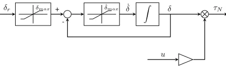
Fig. 2. Steering machine block diagram, representing the relation between momentτN, rudder angleδr, and ship speedu
˙
u= 1
m+Xu˙ h
m(xgr+v)r−DX+τX i
˙
v= 1
m+Yv˙ h
−mur−DY +τY −(mxg+Yr˙) ˙r i
˙
r= 1
−(mxg+Yr˙)2
m+Yv˙ +Iz+Nr˙
"
mxg+Yr˙
m+Yv˙
(19)
mur+DY −τY
−mxgur−DN +τN #
Equation (19) represents the relation between ship control inputs as forces and the accelerations. There is no direct command for lateral forces in an underactuated ship; therefore
τY is set to 0. Longitudinal thrust τX is generated by the ship propellers. In order to produce the desired moment τN, merely commanding the required rudder angle δr, will not change the heading of a stationary ship. In other words, the ship has to be in motion to be able to turn. The moment of ship can be modelled by multiplication of the rudder angle δ and forward speed with a gain. This gain can be identified during sea trials. The rudder has limited speed and cannot respond to the commands immediately. The relation between rudder angle, ship speed, and resulting moment can be considered to be included in characteristics of the steering machine as represented in Fig. 2 [7].
C. Model validation
The parameters required by (19) were set as given in Table I. We used the dimensions and parameters of a scale model with length of1.255[m], which are presented in [8]. The drag coefficients have been calculated based on the ITTC 1957 method [9].
TABLE I. MODEL PARAMETERS
Parameter Value Unit Parameter Value Unit
m 23.8000 [kg] Iz 1.7600 [kgm2]
Xu˙ 2.0000 [kg] Yr˙ 0.0000 [kgm]
Yv˙ 10.0000 [kg] Nr˙ 1.0000 [kgm2]
CX 0.1000 [−] CY 0.5500 [−]
CN 0.0200 [−] xg 0.0460 [m]
Af c 0.0725 [m2] Alc 0.3137 [m2]
[image:7.612.70.303.212.380.2]ye [m]
-10 -5 0 5 10 15 20 25 30
[image:8.612.91.265.52.251.2]xe [m] 0 5 10 15 20 25 30 35 40 45 2 6 10 15 20
Fig. 3. Ship position in Turning circle test for rudder angles of2,6,10,15, and20degrees
tests for ships in sea trials [9]. The experiment was done for the rudder angles ofδ= 2,6,10,15, and20degrees. The test started with propelling the ship in a straight track in the calm water situation. As soon as the ship reached a constant speed
(att= 100[s]), the rudder was turned to the angleδ and was
kept at that position. The rudder command caused the ship to change heading and to start moving in a circle. Fig. 3 illustrates the position of the ship in IF. It can be observed in Fig. 4 that the forward speed drops when the ship starts to turn. Larger rudder angles imply a higher rate of turn, more speed loss, and smaller turning circles.
Therewith, it can be concluded that the developed model manifests results similar to the ones obtained by the Nomoto Model and the experimental data which are presented in [7].
III. CONTROL
In order to facilitate the control action and steering of the ship, three algorithms have been developed, namely, Waypoint generation, Arcs and lines segmented path generation, and Second-order motion profile planning. These algorithms define the control objective and together with feedback and feedfor-ward controllers, they ensure that any maneuvering task can be fulfilled by the ship. In this new approach, the underactuation of the vessel will not hinder the steering performance anymore.
A. Waypoint generation
In practice, ships cannot reach any arbitrary position in workspace with a direct command. For instance, if the desired position is located within a long distance at the back or at the side of the ship, the solution is to take a turn and then head to the target. Achieving this performance only by inputting the final destination would demand complex control methods. We mediate the use of simple PD-controllers by generating waypoints from the starting position of the vessel towards the
0 50 100 150 200 250 300
δ
[deg]
0 10 20
0 50 100 150 200 250 300
r [deg/s] 0 2 4 6 2 6 10 15 20 Time [s]
0 50 100 150 200 250 300
u [m/s]
[image:8.612.322.569.53.250.2]0 0.1 0.2 0.3
Fig. 4. Turning circle test results for rudder angles of2,6,10,15, and20
degrees, Top: Rudder angleδ[deg], Middle: Rate of turnr[deg/s], Bottom: Forward speedu[m/s]
desired point. This decision will simplify the control action significantly.
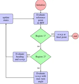
In the developed algorithm, the workspace of the ship has been classified into three regions according to Fig. 5. Region 1 is close vicinity of the ship where it can be accurately positioned with low speed by use of bow and stern thrusters. This region can also be called full actuation area. Region 2 is within maximum turning angle of the ship and the vessel can reach any point in this region with no extra maneuvering. Region 3 is the directly inaccessible area, where the ship should perform extra maneuvers to arrive at a point. Note that in reality, the demarcation lines between Region 2 and Region 3 are curves based on the turning circle of ships; but here a simplified version is employed.
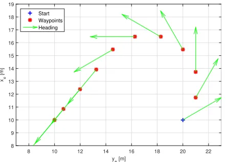
The algorithm starts with receiving information including location and heading of the ship, position of final point, and maximum turning angle. The final point is translated to the body fixed coordinate system and it is decided upon which region it belongs. If the final point is in Region 3, maximum turning will be recommended and the next waypoint will be set such that the target would gradually be placed in region one or two. In case the final point is in Region 2, ship heading will be corrected on demand. The distance between waypoints is set to two times the length of ship according to a convention in marine technology [5]. Generation of waypoints will be continued until the final point is reached.
yb xb
Region 1 Region 2
[image:9.612.367.527.51.253.2]Region 3
Fig. 5. Classification of workspace in BFF into regions; Region 1: full actuation, Region 2: Directly accessible, Region 3: Directly inaccessible
ye [m]
8 10 12 14 16 18 20 22
[image:9.612.92.265.54.230.2]xe [m] 8 9 10 11 12 13 14 15 16 17 18 19 Start Waypoints Heading
Fig. 6. Waypoint generation algorithm results for scaled model. Starting state:(xs, ys, ψs) = (10,20, π/3), desired position:(xd, yd) = (10,10)
B. Arcs and lines segmented path generation
Direct introduction of the waypoints in discrete form to a controller will cause discontinuities and sudden changes in the heading, which are undesired. To avoid this problem, the ref-erence signal should be smooth and continuous. We construct line and arc segments between the generated waypoints as Dubins path, which is the shortest path that connects between two points [10]. Fig. 7 presents the smooth path for generated waypoints extended from(0,0)to(−10,10). The dashed lines in this figure are the circles which form the arc segments.
C. Second-order motion profile planning
Steering a ship towards a desired path or position is done in an over-damped manner; because it is costly and sometimes unacceptable to have any overshoots in position. Adjustment of speed with correct timing is usually done manually and by relying on the experience of ship crew. One way to attain the same performance in an automatic steering system
ye[m]
0 2 4 6 8 10
xe [m] -10 -8 -6 -4 -2 0 2 4 Waypoints Path
Fig. 7. Arcs and lines segmented path generation, starting state:
(xs, ys, ψs) = (0,0,0), desired position:(xd, yd) = (−10,10). The dashed
circles are used to generate the arcs.
is to attribute this over-damped behaviour to the controller. However, this requires a complete knowledge of the system equations and parameters which is not possible in practice.
In order to keep the controller simple and to achieve the desired performance, the position reference is planned as a second-order motion profile. This method leads the ship to a target point with any desired speed. In addition, time is optimized to avoid the disadvantage of slow over-damped sys-tems. The aforementioned features are added to the algorithm presented in [11], where motion planing for point-to-point and standstill to standstill profile has been done.
The motion profile consists of three phases of acceler-ation, constant velocity, and deceleration. The optimization problem can be formulated for three unknowns which are the duration of each phase. These timings should satisfy two requirements for the desired distance and the velocity subject to the constraint of total time of the task. The defined nonlinear multi-variable optimization problem is solved using “fmincon” function from MATLABTM Optimization Toolbox.
Fig. 8 illustrates the planned motion profile for a 50[m]
voyage under 30[s]. Initial speed of the ship is 0.1[m/s] and it is expected to arrive at final point with speed of 0.5[m/s]. The values for acceleration and deceleration are considered
0.6[m/s2]and−0.3[m/s2], respectively. The vessel can reach to the maximum speed of 2[m/s]. The solution provides the best timing and satisfies all the requirements.
[image:9.612.68.289.270.428.2]0 5 10 15 20 25
Position [m]
0 20 40
0 5 10 15 20 25
Velocity [m/s]
0 1 2
Time [s]
0 5 10 15 20 25
Acceleration [m/s
2]
-0.4 0 0.4
Fig. 8. Planned second-order motion profile for50[m]voyage. Top: Position
[m], Middle: Velocity[m/s], Bottom: Acceleration[m/s2], The distance is covered in28[s]
D. Feedback control
In the developed control method, we introduce the path to be tracked by the vessel in BFF. This choice transforms the track-ing problem to a regulation control problem, where the aim is to reduce the distance to reference and the turning to zero. The transformation is done by two-dimensional orthonormal change of coordinates as follows:
PI =HBIPB→PB =HIBPI (20)
P = [x, y,1]T
where I and B stand for IF and BFF, respectively, and P
represents the general motion. HI
B is a homogeneous matrix, which is defined as:
HI
B =
RI B OIB
0 1 (21) RI B=
cosψ −sinψ
sinψ cosψ
, OI
B= x y (22)
The homogeneous matrix should be inverted to obtain the position of any arbitrary point in the BFF:
HIB = (HBI)−1=
(RI
B)T −(RIB)TOBI
0 1
(23)
The control action is done by closing the feedback loop using three PD-controllers with low-pass filters for regulating three signals, namely, longitudinal error, lateral error, and error in the heading. The output of controller in the longitudinal case commands the main propeller’s thrust. The next two control signals are added to suggest the required rudder angle and the corresponding moment. For all controllers, the P and D parameters are tuned based on decoupled simplified models as single-masses so that the open-loop system would have cross-over frequency about 1[rad/s]. The gains are set according
to mechanical specifications to avoid saturation in controllers. Note that there is little need for increasing the type of the system by adding an I-element to this control design, since the constant errors are largely eliminated with a feedforward controller.
E. Feedforward control
The thrust generated by the main propulsion system can be divided into three forces; the force needed to achieve the desired acceleration, the force which overcomes the drag force acting on the ship hull, and the force required to compensate for the errors. The latter is generated by the feedback con-troller. We use the planned acceleration and speed together with weather information and ship parameters to generate an estimate for the first two forces in form of a feedforward controller. This decision provides higher positioning accuracy and better error handling. The following relations are used to calculate feedforward forces:
F Facc= (m+Xu˙)a∗ (24)
F Fvel= 1
2ρAf cCX|v ∗
r|vr∗ (25)
where the asterisks represent the planned variables. It can be seen that only four parameters from the ship specifications are used in the controllers, namely massm, virtual massXu˙, front ship area Af c, and drag coefficientCX. The low number of model variables helps the robustness of the method. If there is uncertainty involved in the parameters, the feedback control should compensate for the differences in forces.
Fig. 9 shows block diagram presentation of the designed control structure. The reference position and heading signals in IF are obtained using the three introduced algorithms. The desired reference position signals in BFF xdb and ydb and heading errorψerrorare generated using feedback from system states. Acceleration and velocity signals are used in feedfor-ward controller. The output of both feedback and feedforfeedfor-ward controllers are added to form the command signals for ship’s thrust and moment. The Ship block in the figure contains the model presented in (19) and Fig. 2.
IV. RESULTS
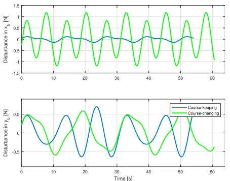
The performance of the developed control method was tested by conducting Course-keeping and Course-changing simulation experiments. Effects of large waves and wind were simulated as multiple frequency sine signals to resemble the forces slamming the ship hull as depicted in Fig. 10. In order to evaluate the robustness of design against uncertainties,10%
[image:10.612.66.287.49.227.2]W aypoint generation Arcs and lines se gmented path generation Second-order motion profile generation Coordinate transfor-mation PDx PDy PDψ FFacc FFvel Ship Starting state + Ending position Waypoints Path Speed in waypoints Disturbances Acceleration Velocity Position Heading xdb ydb ψerror + + + + + Thrust Moment x y ψ
Fig. 9. Control structure overview
0 10 20 30 40 50 60
Disturbance in x
b [N] -1.5 -1 -0.5 0 0.5 1 1.5 Time [s]
0 10 20 30 40 50 60
Disturbance in y
[image:11.612.63.290.260.438.2]b [N] -0.5 0 0.5 Course-keeping Course-changing
Fig. 10. Disturbances as forces inxbandybdirection for Course-keeping
and Course-changing experiments
A. Course-keeping
A straight trajectory was planned to be followed which consisted of the final point at 100[m] as the only waypoint. The ship was continuously exposed to extreme water current perpendicular to the planned voyage with a constant speed of 0.3[m/s] towards east. The ship started from stand-still position and it was planned to reach a forward speed of1[m/s]
at the end of path within 55[sec].
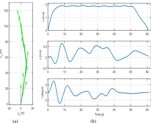
Fig. 11a shows reference path, voyage made by the ship and ship heading. It was observed that the heading (indicated by green arrows) was inclined towards the west. This helped the ship to overcome the lateral force while propelling the body forward. The result was maximum error of 0.5[m]inye direction. As shown in Fig. 11b, the ship follows the planned motion profile to satisfy the forward speed requirements. Side speed and turning rate were influenced by water current and lateral waves and wind. Water current gave a bias to the side speed while the slamming waves sequence could be identified
y e [m]
-10 0 10
xe [m] 0 20 40 60 80 100 120 (a)
0 5 10 15 20 25 30 35 40 45 50 55
u [m/s]
0 1 2
0 5 10 15 20 25 30 35 40 45 50 55
v [m/s]
0 0.2 0.4
Time [s]
0 5 10 15 20 25 30 35 40 45 50 55
r [deg/s]
-5 0 5
(b)
Fig. 11. Course-keeping experiment (a) Reference path, ship voyage and heading (b) Speed in three modes
in the measured speed. The turning rate was higher at the beginning of the motion because of starting in stationery state. This observation implies the necessity of staying above minimum maneuverability speed to ensure full control over ship heading.
B. Course-changing
The aim of the second experiment was to test the ship heading in curved paths with presence of disturbances. The trajectory was planned using one middle waypoint at(50,10)
and the Arcs and lines segmented path generation algorithm. The second-order motion profile algorithm was used to ensure full speed at the given waypoint, best timing, and complete halting at the end of the path. The ship was exposed to head and side waves and water current with speed of 0.1[m/s]
[image:11.612.325.571.270.467.2]ye [m]
-20 0 20
xe [m] 0 20 40 60 80 100 120 (a)
0 10 20 30 40 50 60
u [m/s]
0 1 2
0 10 20 30 40 50 60
v [m/s]
-0.2 0 0.2
Time [s]
0 10 20 30 40 50 60
r [deg/s]
-5 0 5
[image:12.612.56.300.59.258.2](b)
Fig. 12. Course-changing experiment (a) Reference path, ship voyage and heading (b) Speed in three modes
0 10 20 30 40 50 60
Forward thrust [N]
-5 0 5 10 15 Time [s]
0 10 20 30 40 50 60
[image:12.612.65.288.309.485.2]Moment [Nm] -0.4 -0.2 0 0.2 0.4 Course-keeping Course-changing
Fig. 13. Resulting control signals for steering the ship for both Course-keeping and Course-changing experiments
Fig. 12a manifests the performance of the ship in this scenario; the path was followed with correct heading, and the environmental disturbances did not deviate the ship. Maximum lateral error was 0.7[m], which occurred during the course changing. Speed was measured as shown in Fig. 12b. The fluc-tuations in forward speed were caused by the heading waves. Side speed and turning rate were influenced by curvature of the path and also external side forces.
Fig. 13 compares the resulting control signals for steering the ship in both experiments. It was assumed that the scaled model used in the simulations could apply thrust and moment limited to [−5,15][N]and[−0.5.0.5][N m], respectively.
V. CONCLUSION
In this paper, we addressed the problem of steering under-actuated ships subject to various disturbances. A model was developed based on the ship hydrodynamics. Validity of the model was shown by running Turning circle experiment. The contribution to the control problem was made from a novel perspective. First, the control objective was redefined to suit the limitations of an underactuated ship. This remedy involved generating waypoints and developing continuous trajectories to ensure that every point in workspace is accessible by the ship. Speed along the path was planned by a time-optimized second-order motion profile to accommodate the over-damped behaviour of ships. Our method was also able to satisfy the speed requirements upon arrival. We changed the tracking problem to a regulation problem in an innovative approach by defining the reference signals in Body Fixed Frame. This choice allowed the use of linear feedback controllers in the next stage. Simple PD-controllers were employed to com-pensate for the position and heading errors. Better accuracy and disturbance rejection was achieved by adding feedforward controllers based on weather data and motion profile. Our control method was tested during two simulation experiments by commanding the ship to follow trajectories in extreme environmental conditions. The tasks were done by engaging the introduced algorithms to compute the desired path, timing, and speed. There was no need for task-based fine-tuning of the PD-controllers and the same controller setting was used in both experiments. The robustness of control design was asserted by adding mismatch between the provided weather information and simulation conditions. All in all, the behaviour of the developed automatic steering control is quite satisfactory.
REFERENCES
[1] Z. Vukic and B. Borovic, “Guidance and control systems for marine vehicles,” inThe Ocean engineering handbook, 2000.
[2] F. J. Velasco, E. Lopez, T. M. Rueda, and E. Moyano, “Ship steering control,” inAutomation for the Maritime Industries, 2004.
[3] K. Nomoto, T. Taguchi, K. Honda, and S. Hirano, “On the steering qualities of Ships,” inInternational Shipbuilding Progress, 1957, vol. 4. [4] T. I. Fossen, “A survey on nonlinear ship control: from theory to practice,” inProceeding of the 5th IFAC Conference on Manuevering
and Control of Marine Craft, 2000.
[5] T. Fossen, Handbook of Marine Craft Hydrodynamics and Motion
Control. John Wiley and Sons, 2011.
[6] K. D. Do and J. Pan,Control of Ships and Underwater Vehicles: Design
for Underactuated and Nonlinear Marine Systems. Springer, 2009.
[7] J. van Amerongen, “Adaptive steering of the ships,” Ph.D. dissertation, Delft University of Technology, 1982.
[8] P. V. K. Roger Skjetne, Thor I. Fossen, “Adaptive maneuvering, with experiments, for a model ship in a marine control laboratory,”
Automatica, vol. 41, pp. 289–298, 2005.
[9] V. Bertram,Practical Ship Hydrodynamics. Butterworth-Heinemann, 2000.
[10] L. E. Dubins, “On curves of minimal length with a constraint on average curvature, and with prescribed initial and terminal positions and tangents,”American Journal of Mathematics, vol. 79, no. 3, pp. 497–516, Jul. 1957.
[11] P. Lambrechts, M. Boerlage, and M. Steinbuch, “Trajectory planning and feedforward design for electromechanical motion systems,”Control
APPENDIXA
[image:13.612.86.252.529.650.2]WAYPOINT GENERATION ALGORITHM BLOCK DIAGRAM Fig. 14, represents the graphical interpretation of the Way-point generation algorithm, which has been explained in sec-tion III.
APPENDIXB
ARC AND LINES SEGMENTED PATH GENERATION PROCEDURE
The algorithm starts with receiving waypoints and starting position of the vessel. The number of required segments is calculated and the lines between each two consecutive waypoints are found. Circles with defined radius are formed around each waypoint. This radius should be chosen according to the ship’s specifications. A small radius would result in sharper corner which might hinder the ship turning, whereas a bigger circle would generate a smoother path but larger deviation from waypoint. Next, the intersection points of the circles and the connecting lines are found. This results in two intersection points per each waypoint. The lines perpendicular to the connecting lines are found at these intersection points. The points where these perpendicular lines meet, are centers of the circles which form the arc segments. At this point, all the arc and line segments are defined. Next step is to form a continuous path with these arcs and lines. Starting from the given position of the ship, the algorithm moves towards the next waypoint until the final point is reached. Whenever a waypoint is met the algorithm toggles between line and arc segments.
The output of this algorithm is the position of the points on the path in IF, which are close enough to resemble a continuous path.
APPENDIXC
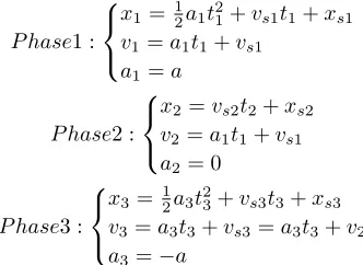
SECOND-ORDER MOTION PROFILE GENERATION The second-order motion consists of three phases: accel-eration, constant velocity and deceleration. The maximum velocity and rate of change of speed while accelerating and decelerating are calculated according to the ship dynamics. The kinematics of voyage can be written as following:
P hase1 :
x1= 12a1t12+vs1t1+xs1
v1=a1t1+vs1
a1=a
P hase2 :
x2=vs2t2+xs2
v2=a1t1+vs1
a2= 0
(26)
P hase3 :
x3=12a3t32+vs3t3+xs3
v3=a3t3+vs3=a3t3+v2
a3=−a
where vs∗ and xs∗ stand for the velocity and position in
the beginning of each phase. Assuming the time limit of tl for reaching the final point, following optimization problem
with three unknowns, two equations and one constraint can be formulated:
∆x=1
2a1t 2
1+ +vs1t1+a1t1t2+vs1t2+ 1 2a3t
2
3+a1t1t3+vs1t3
∆v=a1t1+a3t3
t1+t2+t3< tl
which ∆x=xe−xs1 and ∆v=ve−vs1 are defined. After simplifying the expressions the final optimization problem should be solved to obtain the time period for each frame:
∆x= 12a(t2
1−t23) +vs1(t1+t2+t3) +at1(t2+t3) ∆v=a(t1−t3)
t1+t2+t3< tl
(27)
APPENDIXD PD-CONTROLLER TUNING
The PD-controllers were designed in the frequency domain by using bode plot of the open-loop system. For this purpose, the plant was assumed to be decoupled and it was considered as a single mass in every mode. The relations between the control inputs and the state variables in (19) can be obtained as following:
˙
u= 1
m+Xu˙X
˙
v=−(mxg−Yr˙)
m+Yv˙
1 −(mxg−Yr˙)2
m+Yv˙ +Iz+Nr˙
N (28)
˙
r= 1
−(mxg−Yr˙)2
m+Yv˙ +Iz+Nr˙
N
We write the Laplace transformation of (29) and substitute parameters from Table I. In the following equations, X(s),
Y(s), andΨ(s)denote Laplace transformation ofx,y, andψ, respectively; whereas,F(s)andN(s)are Laplace transforma-tions of forward thrust, X and moment,N.
X(s) = 1 25.8s2F(s)
Y(s) =− 1
84.1153s2N(s) (29)
Ψ(s) = 1
2.7245s2N(s)
Equation (29) is comparable to transfer function:
G(s) =X(s)
F(s) = 1
ms2 (30)
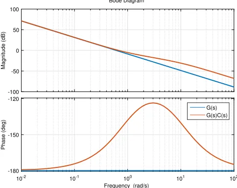
Bode plots for the three presented transfer functions are presented in Fig. 15 - 17. Low frequency behaviour of ship model can be observed according to the cross-over frequencies, which are less than1[rad/s] for all modes.
Initialize
Evaluate reference point in BFF
Region 1? final pointn.w.p at end
Region 2?
Evaluate n.w.p with
max turn angle Evaluate
heading and n.w.p update
states
yes
no
[image:14.612.189.447.55.330.2]no yes
Fig. 14. Waypoint generation algorithm,*n.w.p: next way point
Magnitude (dB)
-150 -100 -50 0 50 100 150
10-3 10-2 10-1 100 101 102
Phase (deg)
-180 -150 -120 -90
G(s) G(s)C(s) Bode Diagram
Frequency (rad/s)
Fig. 15. Bode plot, transfer function G(s) and controller with transfer functionG(s)C(s)inxmode
C(s) =P+ sDs
N + 1
(31)
Magnitude (dB)
-150 -100 -50 0 50 100 150
10-3 10-2 10-1 100 101 102
Phase (deg)
-180 -150 -120
G(s) G(s)C(s) Bode Diagram
[image:14.612.323.566.371.561.2]Frequency (rad/s)
Fig. 16. Bode plot, transfer function G(s) and controller with transfer functionG(s)C(s)inymode
We define:
τ= 1
N
a2= 1 +
[image:14.612.54.296.371.561.2]Magnitude (dB) -100 -50 0 50 100
10-2 10-1 100 101 102
Phase (deg) -180 -150 -120 G(s) G(s)C(s) Bode Diagram
[image:15.612.54.296.56.248.2]Frequency (rad/s)
Fig. 17. Bode plot, transfer function G(s) and controller with transfer functionG(s)C(s)inψmode
Equation (31) can be written as:
C(s) =Kaτ s+ 1
τ s+ 1 (32)
In all three cases the cut-off frequencies were chosen around
1[rad/s] to resemble the low frequency behaviour of ships. Phase margins were selected big enough to ensure system stability, while keeping the bandwidth small enough to reject any high frequency signal. After calculating the controller pa-rameters in frequency domain, simulations were done using the ship model. In some cases, the gains were reduced to comply with mechanical considerations and to avoid saturation in the actuators. However, by trying different values it was observed that the discrepancy from the selected value did not cause large errors. Bode plots of the open-loop systems consisting of the transfer functions and controllers are illustrated in Fig. 15 -17.
It is important to note that the same controllers were used for Course-keeping and Course-changing experiments in section IV. It can be concluded that as long as the controller parameters provide low cross-over frequency and low gain, the response is not sensitive to model specifications and external disturbances.
[image:15.612.323.569.102.295.2]Fig. 18 and 19 present output signals of the designed feedback and feedforward controllers in Course-keeping and Course-changing tests, respectively. In these figures, two sit-uations are compared: 1. there is a mismatch according to Table II between weather data used in feedforward calculations and simulation environment. 2. correct weather data is used. Measured positions in two situations are illustrated in Fig. 20 and 21. It can be observed that there is no considerable difference in the followed path, which implies correct action of PD-controllers.
0 10 20 30 40 50
FF acc [N] -10 0 10 20
0 10 20 30 40 50
FF vel [N] 0 5 10 15
0 10 20 30 40 50
PD x [N] 0 2 4
0 10 20 30 40 50
PD y [N] -0.2 0 Time [s]
0 10 20 30 40 50
PD ψ [Nm] 0 0.2 mismatch correct
Fig. 18. Course-keeping experiment, Output signals of the controllers
0 10 20 30 40 50 60
FF acc [N] -10 0 10 20
0 10 20 30 40 50 60
FF vel [N] 0 5 10 15
0 10 20 30 40 50 60
PD x [N] 0 2 4
0 10 20 30 40 50 60
PD y [N] -0.4 -0.20 0.2 Time [s]
0 10 20 30 40 50 60
PD ψ [Nm] 0 1 2 mismatch correct
[image:15.612.324.569.424.617.2]TABLE II. INFLUENCE OF ERRONEOUS WEATHER DATA
Water current Real values Values in calculations Speed[m/s] Heading[deg] Speed[m/s] Heading[deg]
Course-keeping 0.3 90 0.25 100
Course-changing 0.1 145 0.2 130
0 10 20 30 40 50 60 70
x [m]
0 20 40 60 80 100
0 10 20 30 40 50 60 70
y [m]
0 2 4 6 8 10
[image:16.612.53.297.162.354.2]mismatch correct
Fig. 20. Course-keeping experiment, measured position
0 10 20 30 40 50 60 70
x [m]
0 20 40 60 80 100
0 10 20 30 40 50 60 70
y [m]
0 2 4 6 8 10
mismatch correct
[image:16.612.55.298.445.637.2]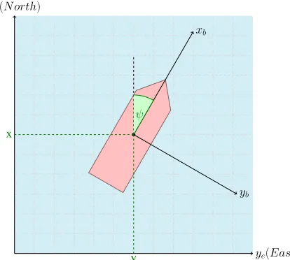
![Fig. 4.Turning circle test results for rudder angles ofForward speed 2, 6, 10, 15, and 20degrees, Top: Rudder angle δ[deg], Middle: Rate of turn r[deg/s], Bottom: u[m/s]](https://thumb-us.123doks.com/thumbv2/123dok_us/9791762.480338/8.612.322.569.53.250/turning-circle-results-rudder-offorward-degrees-rudder-middle.webp)
![Fig. 8.Planned second-order motion profile for[covered in 50[m] voyage. Top: Positionm], Middle: Velocity [m/s], Bottom: Acceleration [m/s2], The distance is 28[s]](https://thumb-us.123doks.com/thumbv2/123dok_us/9791762.480338/10.612.66.287.49.227/planned-prole-covered-positionm-middle-velocity-acceleration-distance.webp)