Frequency tagging of electrocutaneous stimuli for observation of cortical nociceptive processing

(1)

26 June 2016

BACHELOR ASSIGNMENT

FREQUENCY TAGGING OF

ELECTROCUTANEOUS STIMULI

FOR OBSERVATION OF CORTICAL

NOCICEPTIVE PROCESSING

S.F.J. Nijhof

s1489488

Faculty of Electrical Engineering, Mathematics and Computer Science (EEMCS) Biological Signals and Systems (BSS)

(2)

(3)

Summary

Research on nociceptive (pain related) processing in the human nervous system is required to improve treatment for chronic pain patients. A key characteristic of chronic pain is develop-ment of maladaptive nociceptive processing. If these changes could be detected in an early stage, more accurate treatment could be given and would yield better results and less clinical effort per patient. Diagnostic methods are useful for characterizing the processing of nocicept-ive information. Observation methods have been developed already to measure responses to phasic stimuli applied to the peripheral nervous system. In combination with EEG measure-ments, more objective information can be obtained. Previous methods show good results in observation of neural responses to stimuli. This would be improved by an possibility to meas-ure neural measmeas-urements of longer durations.

New investigations are carried out aimed to evaluate responses of longer lasting tonic stim-uli. ’Frequency tagging’ is a method that could be used for this. With frequency tagging, a pulse train of several seconds with pulses in the millisecond range is modulated on and off with a certain specified frequency. The goal of applying stimuli with this pattern is to see this same modulation frequency back in measurements of specific activated places in the bran corres-ponding to nociceptive processing. In this assignment, frequency tagging is implemented on a setup that was able to send phasic stimuli only. Key factor in the design of this setup is the strict timing requirement for generation of accurate frequencies. Properties related with timing are first evaluated, thereafter a validation experiment of the entire setup was performed. This validation experiment was done on a human subject. A relative nociceptive threshold was de-termined by applying pulse trains with increasing amplitude while measuring reactions. After the threshold was determined, the pulse train amplitude was set to twice this value to generate a definite pain sensation. Pulse trains with modulation frequencies of 13, 20, 33 and 43 Hz were applied and EEG was measured. Phase locked and non phase locked analysis in time and frequency domain was performed to interpret the data.

Results show that frequency content corresponding to the input signal can be found back in the EEG measurements. Specific sharp peaks are observed in the frequency-magnitude plot of EEG channel derivations. Frequencies at which these peaks occurred where higher har-monics and combinations of the modulation frequency and frequency corresponding to single pulse timing. Phasic responses were found at the onset of pulse trains. Frequency content at the modulation frequency was only found for 33 Hz. For all other modulation frequencies, the fundamental frequency could not be observed clearly. Evaluating at 50 ms time around stim-ulus onset specifically, it was found that frequency content corresponding to the input signal was measured in EEG signals before human responses were possible. This is an indication of stimulus artifacts in the measurements.

(4)

Abbreviations

EEG Electroencephalography ES Electrical stimulation DFT Discrete Fourier transform FFT Fast Fourier transform

fMRI Functional magnetic resonance imaging IES Intra-epidermal stimulation

IPI Inter pulse interval

MEG Magnetoencephalography MWT Morlet wavelet transform NoP Number of pulses LS Laser stimulation

PET Positron emission tomography PSD Power spectral density

(5)

1. Introduction

1.1 Context

Annually 150.000 to 200.000 patients suffer from chronic pain in the Netherlands. Once a person has chronic pain, relatively ineffective treatment is performed. To make treatment bet-ter, diagnostics and therapeutic measures in an early stage would result in better treatment outcome and less clinical effort per patient. Chronic pain is often the result of disturbed pro-cesses in the central nervous system. An increased sensitivity to noxious stimuli (generalized hyperalgesia) is widely recognized as key factor in chronic pain development. Nociceptive stimuli are processed by neural mechanisms at several places in an ascending pathway from the peripheral nervous system to the brain, resulting into conscious experience of pain. The ascending processing is modulated by descending pathways. Due to injury or disease, mal-adaptive changes in both ascending and descending pathways may result in increased pain sensitivity. Clinical observation methods of maladaptive processing are limited at this moment, but if insight would be increased this would permit better understanding and early detection of chronic pain.

1.2 Previous findings

(8)

1.3 Research objective

The goal of this bachelor assignment is to implement a frequency tagging measurement setup. Hardware of an existing nociceptive threshold tracking setup will be used as a starting point. This can be extended with different software while hardware can be kept the same. After im-plementation of the setup, a first experiment will be carried out in such a way that a preliminary data analysis can be executed. Results could then be used as a validation method for the extension of the measurement setup. If the setup would be correct, results could also be used for characterization of nociceptive processing pathways.

1.4 Report structure

(9)

2. Theory

In order to design a device which is intended to characterize the human body, it is necessary to know what needs to be characterized. Therefore, a literature study on nociceptive processing in the human body will be needed. To be able to present stimuli to and obtain responses from the human body it has to be known which methods are available, therefore the literature study will cover neurostimulation methods and EEG analysis methods as well. Methodologies and results of previous work covering frequency tagging of nociceptive pathways will also be discussed to generate initial sense of the methodology.

2.1 Nociceptive processing

One of the functions of the nervous system is managing transport of signals to different parts in the body. Sense and motor organs are all connected with the nervous system in the human body to send and receive signals. One type of sense organs in the skin are nociceptors. Nociceptors are spread over the whole body and are responsible for sensing pain. Signals originating from these receptors are processed in an ascending pathway via afferent nerve fibers in the peripheral nervous system, laminae in the spinal cord, centers in the brainstem and thalamus to the primary somatosensory cortex in the brain. Different descending pathways exist as well, these have ability to modulate the ascending pathway signal transmission. Since nociceptive processing will be discussed superficially here, main reasoning in this section is followed from introductory text books from Purves et al. [1] and Noback et al. [2]. As an electrical engineering student, this is not general accepted knowledge but for persons with a medical background it should be.

2.1.1 Sensory receptors in the skin

There are different types of sensory receptors in the skin, based on function they can be cat-egorized into three groups: mechanoreceptors, nociceptors and thermoceptors [1]. Mechanor-eceptors are mainly in the deeper layers of the skin. Nociceptors and thermoceptors can also be found in the upper regions of the skin. This is because both receptors are different types. Nociceptors and thermoceptors are free nerve endings and mechanoceptors have specific receptor elements. The free nerve endings are branches from neurons and can convert stim-ulation directly into action potentials. If a nerve ending is stimulated, the permeability of the cell membrane is changed. This results in a depolarizing current going to the central nervous system. Strength of a stimulus is non linearly related to different rates of action potential that are generated by receptors. This process is different per type of receptor. Due to difference per receptor, information can reach the brain quick if a strong stimulus is present and information can reach the brain when a stimulus is going on for a longer time. Phasic receptors can adapt their output relatively fast and respond with a maximal rate of action potentials for a short time and tonic receptors adapt their output slower but keep firing at a lower rate and keep going for a longer time. Nociceptive receptors can be seen as tonic receptors.

(10)

[image:10.595.181.415.50.448.2]

Figure 2.1: schematic representation of nociceptive pathways. From [2].

velocities of signals. Nociceptors attached to the different fibers react to different stimuli. Aδ -fibers have low-threshold receptors and corresponding signals are felt as sharp stinging pain, C-fibers have high threshold and give signals corresponding to widespread pain that might be felt as burning or itching [2].

2.1.2 Ascending pathway

Signals created by nociceptive nerve fibers are transmitted to corresponding neurons lying in dorsal root ganglia, see figure 2.1. These neurons then enter the spinal cord via dorsal roots. The axons of neurons that enter the spinal cord split into branches that ascend and descend one to two spinal levels. This forms the dorsolateral tract of Lissauer [1][2]. These branches enter and terminate in the grey matter of the dorsal horn. Here the branches pass the signal to several Rexed’s laminae. Fibers of each part of the body join at higher levels of the spinal cord and result in a separated projection.

(11)

secondary somatosensory cortex. Nociceptive information in these areas is thought to be identifying location and intensity of pain as well as quality of the stimulation [1]. Other areas in the brain are responsible for psychological modulation of pain perception. The insular cortex and anterior cingulate cortex are involved with judging the intensity of pain [3][4].

2.1.3 Modulation of nociceptive information

Nociceptive information that ascends to cortices is modulated by descending signals which can both inhibit or facilitate the sensitivity of nociceptors and processing centers of pain in the central nervous system. Signals can originate from the somatosensory cortex, amygdala and hypothalamus and go to the periaqueductal grey in the midbrain in the brainstem [1][5]. Stimulation of the periaqueductal grey is processed via different centers in the brainstem to the descending pathways in the spinal cord. The different centers in the brainstem are respons-ible for generating multiple different neurotransmitters which can have positive and negative effects. These neurotransmitters affect descending pathways in the spinal cord as well as con-nections between ascending and descending pathways and synaptic terminals of nociceptive afferents [1]. It is also possible for neural circuits within the dorsal grey in the spinal cord to modulate information of nociceptive afferents such that higher centers already receive modu-lated information.

2.1.4 Maladaptive neural processing

There are a lot of ways in which the processing of nociceptive information can be affected and not all of these are known. One of many consequences of maladaptive neural processing is chronic pain. This could be caused by changes in the working of descending modulation net-work [6], for instance due to an operation. Patients could have either an insufficient descending inhibitory system or an enhanced descending facilitatory system. Since the descending path-way in the spinal cord is controlled by centers in the brainstem, it has been shown that different centers in the brainstem can have positive or negative effects on central sensitization and hy-peralgesia [6]. This results in an increased sensitivity and possible persistence of pain and are key indicators for chronic pain.

2.2 Neurostimulation methods

2.2.1 Stimulation methods

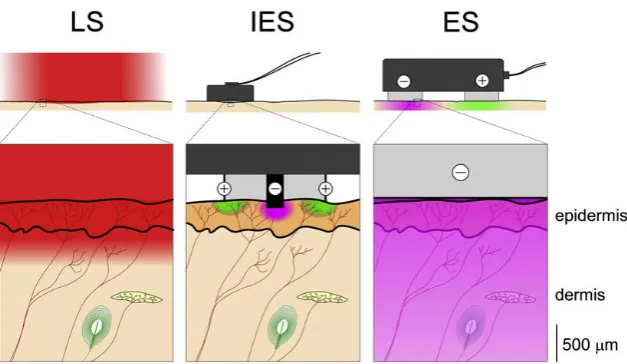
In order to activate nociceptive processing, the body has to be stimulated. It is important that such stimuli generate the same response of the nervous system as what would happen when a normal painful event occurs. It is also important that nociceptive nerves can be stimulated se-lectively in order to characterize pathways of nociceptive information separately from pathways of other non-nociceptive mechanisms. The purpose of stimulating the nerves is to measure nociceptive pathways. This means that a measured response should be linked to a certain stimulus. Such a relation between stimulus and response requires strict time requirements of the stimulator. For example, if stimuli are presented with a too slow increase of amplitude, it is not certain what provoked a response. Three different stimulation methods are described here: laser stimulation (LS), intra-epidermal stimulation (IES) and transcutaneous electrical stimulation (ES). The methods are schematically represented in figure 2.2 and explained fur-ther below.

(12)

[image:12.595.141.455.49.231.2]

Figure 2.2: schematic overview different stimulation methods. Laser stimulation (LS), intra-epidermal electrical stimulation (IES) and transcutaneous electrical stimulation (ES) are represented. Only Aδand C nociceptive-free nerve endings can be found in the most superficial layers of the skin. Non-nociceptive receptors are located deeper. From [7].

generate steep heating ramps which result in time-locked responses in the brain [9], however additional time is required for heat conduction to the skin and transduction into a neural im-pulse. A disadvantage of laser stimulation is that time between two stimuli at the same location should be long (usually 5-20 seconds) and skin temperature cannot be controlled by solely the laser [8].

Second, a method to activate nociceptors selectively is by intra-epidermal electrical stimulation (IES). This method is based on a separation between nociceptive receptors in the epidermis and non-nociceptive receptors in the dermis. Small currents spatially restricted to the epi-dermis are applied via a small flat needle. For low currents, only the epiepi-dermis is affected and IES is shown to be selective for Aδ-fibers [7]. Small currents might not be strong enough for generating a good perception or signal to noise ratio. Temporal summation can be used to compensate for that. This is done by using short IES pulse trains, where longer pulse trains result in higher intensity of perception and higher amplitude of evoked potentials (EP) in the brain [10][11].

Third, a crude stimulation method named transcutaneous electrical stimulation (ES) can be used. This method delivers a current to the epidermis and dermis, resulting in activation of non-nociceptive and non-nociceptive receptors. Most non-non-nociceptive receptors have lower thresholds than nociceptors [1]. This means that non-nociceptive are activated more if a stimulus is ap-plied. Due to activation of non-nociceptive receptors, this method is not selective for nocicept-ors and thus not suited for characterizing nociceptive pathways.

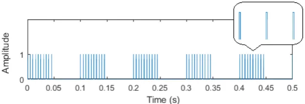
2.2.2 Stimulus content

(13)

[image:13.595.142.455.56.163.2]

Figure 2.3: square wave modulated pulse train.

nervous pathway exists. A name used to describe this method is frequency tagging. Success-ful previous frequency tagging research has been done by characterization of visual neural pathways [14][15], tactile neural pathways [15][16] as well as nociceptive pathways [15][17]. Considering frequency tagging for nociceptive pathways, different frequencies have been used for characterization (3-43 Hz). This is relevant since neural pathways could react different to different frequencies. The applied stimulus pattern was always a train of equal fixed amplitude pulses modulated by a lower frequency, 50% duty cycle square wave, as can be seen in figure 2.3. This is something that could be elaborated on. The amplitude could be varied but if IES is used this has negative consequences for selectivity of nociceptors. For short pulse trains (1-5 pulses) it has been shown that more pulses result in a higher intensity of perception and higher amplitude of evoked potentials in the brain [10][11]. An elaboration on this could potentially be used for frequency tagging. The intensity of stimuli could be varied by changing the duty cycle of the modulating square wave. Another elaboration would be to apply a temporal signal that is modulated with multiple known frequencies such that one measurement that includes different frequencies can be done at once.

2.3 Similar work

Frequency tagging experiments with nociceptive stimuli has already been done by Colon et al. [17]. Here, experiments were done to compare EEG measurements on both hands of a human subject. Tonic non-nociceptive ES stimulation of Aβ-fibers and tonic nociceptive IES stimula-tion of aδ-fibers was performed. The stimulation procedure consisted of 5 blocks of 10 pulse trains lasting 10 seconds. Pulses had a width of 0.5 ms and were separated by 5 ms. Used modulation frequencies were 3, 7, 13, 23 and 43 Hz. The pulse amplitude of IES stimulation was determined by twice the measured nociceptive threshold of a single 0.5 ms pulse.

Data analysis was done by first applying a 0.5-250 Hz band pass filter to all signals. Non overlapping EEG segments were obtained from 0 to 10 seconds during the stimulation. Each segment was demeaned and eye blinks were removed by independent component analysis. Epochs with artifacts larger than 500µV were removed. Non phase locked analysis was per-formed on averaged waveforms. Additional noise was removed by subtracting a relative aver-aged amplitude from frequencies in smaller range than 0.5 Hz.

(14)

2.4 Analysis methods

2.4.1 Electroencephalography

Cortical activities are needed to be measured in order to be able to see cortical responses to given stimuli. Various methods exist to measure activity in the brain, for example positron emission tomography (PET), functional magnetic resonance imaging (fMRI), magnetoenceph-alography (MEG) and electroencephmagnetoenceph-alography (EEG). The latter option is widely used because of ease of use, mobility, possibility of long time monitoring and, more importantly, EEG is based on measuring electric potentials which are primary effects of neural excitation, while metabolic changes in the brain tissue measured by PET or fMRI are secondary effects [18]. Therefore, EEG has much more resolution in the time domain, which means that it is better suited for measuring rhythmic activities. A disadvantage of EEG is that the resolution in spatial domain is limited, e.g. a limited amount of electrodes can be present. If resolution in the spatial domain is needed, MEG is advantageous with respect to EEG, since magnetic fields are less distorted than electric fields by the skull and scalp, resulting in a better spatial resolution. However, EEG is able to record radially oriented dipoles, which is something that MEG cannot do [19]. Considering all cons and pros of each method, EEG is considered best to work with.

2.4.2 EEG data analysis

Electrodes are placed on the scalp in order to measure cortical activities using EEG. These electrodes usually cover across the whole scalp, but only information from certain positions is necessary since there is only interest in areas involved with nociceptive processing. It would be expected that areas as somatosensory cortex I and II are reacting most heavily on nociceptive stimuli. The locations of these cortices are in the parietal lobe, just posterior to the central sulcus. Electrode placement to measure these areas, according to the 10-20 system, would be C4-Fz or C3-Fz contralateral to the stimulated side and Cz-M1M2. These measurements locations have been successful in previous research into temporal properties as well [11][13]. Other research related to frequency tagging found electrode pairs C4-Fz or C3-Fz contralateral to the stimulated side to be successful [20][17].

The acquired signal after EEG measurement will contain noise, which is not desired. After the measurement, signal processing can be done to analyze signal properties. Several tech-niques exist to remove this noise. First, the signal can be band pass filtered to the frequency band relevant for research. For purposes of understanding it would be convenient to keep the bandwidth rather broad, such that frequencies nearby the stimulus frequency are kept. Second, similar segmented time signals with respect to stimulus onset can be averaged in time to reduce noise. However, the time signal contains signal amplitude and phase informa-tion. This means that if two signals would be in antiphase in the same time interval, they would cancel out each other. If the average signal would be transformed to frequency domain, it is called a phase locked analysis. A signal could also first be transformed to frequency domain, after which only the amplitude information can be averaged. Such an analysis is a non-phase locked analysis. Differences between the two could indicate strength of signals phase locked to the stimulus. Third, a part of the noise is present from artifacts of other activities such as eye blinking and heartbeat. By using a blind source separation by independent component analysis, it is possible to remove these artifacts [21]. Another way to overcome this problem is rejecting all EEG epochs containing artifacts larger than an arbitrary chosen threshold, how-ever by applying this technique a part of the measurement data is lost.

(15)

transform (DFT). A DFT is a purely mathematical operation, but with the DFT the power spectral density (PSD) can be calculated as well. The PSD describes how signal power is distributed over frequency. The measurable frequencies are triggered at a certain point in time. It would be advantageous to see which frequency is available at which point in time to analyze frequency components during and after the onset of a stimulation. To view information in both time and frequency domain, a Morlet wavelet transform (MWT) can be done. With the MWT it is possible to plot the signal as function of time and frequency, where resolution is divided between the two.

2.5 Discussion

2.5.1 Stimulation methods

Different methods of stimulating nociceptive receptors have been given. Laser stimulation and intra epidermal electrical stimulation are suitable for selective stimulation of Aδ-fibers. From these two options, IES is more practical and is more widely used in literature and will therefore be chosen to work with.

2.5.2 Stimulus content

A certain modulated pulse train will be used to stimulate subjects. The work discussed in section 2.3 can be used as indication for suited modulation frequencies. Properties of single pulses could be based on these findings as well, however experiments with the specific setup that will be described in chapter 3, different pulse properties might give better results.

2.5.3 EEG processing

(16)

3. Design

Literature study as described in chapter 2 reveals how nociceptive processing is taking place in the human nervous system and how a measurement setup could interface with the human body. In this chapter the design of the measurement setup will be described. A measurement setup that can give stimuli and measure EEG of the scalp and conscious pain experience is already available and will be elucidated. This existing setup has to be modified to be able to perform frequency tagging experiments. The modification will be done by specifying re-quirements and building corresponding implementations. To test and validate the changes, a validation experiment will be described.

The existing measurement setup was built to carry out experiments which tracked nociceptive thresholds for different stimuli [12][13][22]. The corresponding software of the controlling PC is based on LabVIEW 2013 SP 1. This software controls and registers the to be applied stimulus amplitudes, the response to stimuli and the time at which a stimulus is given. A response to stimuli was indicated via a button by whether or not the person felt the stimulus. Another PC was used for the recording of amplified EEG signals.

Hardware used for tracking of the nociceptive threshold can be found schematically in fig-ure 3.1. The controlling PC is connected via a parallel 8-bit trigger cable to an EEG amplifier (ANT Neuro 64-channel Refa-72), such that another PC capturing EEG data can store cor-responding stimulus data with EEG data. 6 bits of the trigger cable are for stimulus amplitude information and 2 bits are for temporal stimulus settings. If any trigger code is present, a 1-bit trigger signal will be send to the stimulator (NociTRACK AmbuStim) and the stimulator will stimulate the corresponding stimulus. This stimulator has a Bluetooth connection with the con-trolling PC such that stimulus information can be send to the stimulator and human responses can be send to the controlling PC. Stimulation is done using an IES electrode consisting of a pad with five needles for preferential stimulation of Aδnerve fibers [23]. The actual stimulation amplitude differs from the desired stimulation amplitude, therefore every stimulator has to be calibrated. This is done with software using linear regression.

3.1 Requirements for frequency tagging

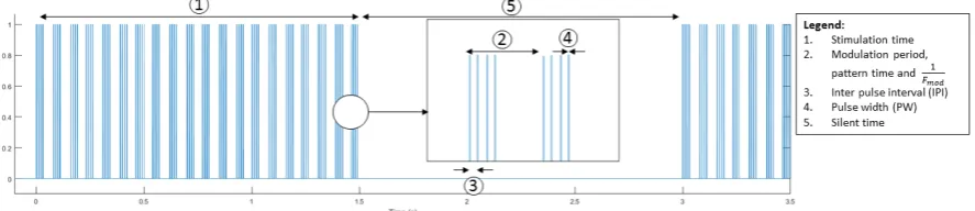
The existing measurement setup has to be changed to implement frequency tagging. The idea is to stimulate a person with tonic stimuli from which the frequency is known and between 10 to 50 Hz. To be able to stimulate with precise frequencies, timing of pulses and inter pulse interval is crucial. The main adaptations have to be made in the control PC which generates the stimulus patterns for the stimulator.

The new setup should be able to send controlled timed pulse trains for several seconds in-stead of one pulse every few seconds. Several settings of the applied tonic stimuli should be changeable. Definitions of names for timing can be found in figure 3.2. Stimulation time (s), modulation frequency (Hz), IPI (ms), PW (ms) and silent time (time until next stimulation time in s) are all parameters that can be set to carry out the desired experiments. These settings should lead to correct behavior of the stimulator.

(17)

[image:17.595.188.409.53.266.2]

Figure 3.1: hardware setup consisting of a controlling PC, EEG recording PC, stimulator, stimulation electrode, EEG measurement cap and EEG amplifier. From [13].

different skin conditions. It would be better to set the amplitude with reference to a nocicept-ive threshold. Previous experiments were already indicating nociceptnocicept-ive thresholds for phasic stimuli. However, if tonic stimuli are used in the actual experiment, the threshold is different from single pulses. Only the probability of detection when multiple pulses are used is already higher than detecting a single pulse with the same amplitude. Nociceptive nerves could also react different to tonic and phasic stimuli. Therefore, a threshold determining experiment for tonic stimuli should be set up. One way to determine this threshold is by a so called staircase procedure. With this procedure, the amplitude keeps increasing until the person feels a stim-ulus. This procedure could be set up by repeating the same settings as the actual frequency tagging experiment for a very short time and an increasing amplitude, meanwhile the program is keeping track of the average nociceptive threshold.

3.2 Frequency tagging implementation

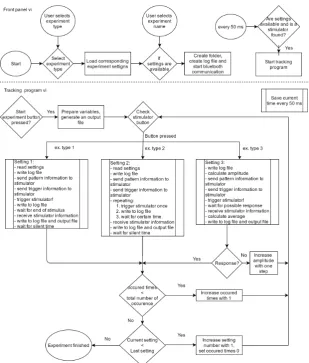
The main adaption of the current measurement setup is done on the software of the controlling PC. The software has to process a given settings file to control the stimulator, give trigger codes to the EEG amplifier and stimulator and keep a log file during the experiment. The log file is keeping track of the program status and is giving information about given stimulations. Another file is created as well. This file is the settings file with additional information about timing and trigger codes gathered during the executed experiment and is used for data analysis later. A flowchart is made to give an overview of the main functionalities of the program. This can be found in figure 3.3.

[image:17.595.78.522.663.759.2]

(18)

[image:18.595.141.451.49.413.2]

Figure 3.3: flowchart of the main functionalities of the stimulation PC program for fre-quency tagging experiments.

3.2.1 Stimulator control

(19)

end of the duty cycle. The calculation for number of pulses can be found in equation 3.1. Here, the division is rounded down to the nearest integer, since it is only possible to have an integer amount of pulses. Because the result is always an integer, the duty cycle is slightly lower than 50% in some cases. The inter pulse interval is different for different pulses in one period of modulation frequency. All pulses except the last one keep the initially specified IPI. The last pulse is specified with a longer IPI to create a silent time in the last half of the modulation period. Calculation of the last IPI can be found in equation 3.2. Correction factors are added at the calculation of IPI and NoP to go from seconds to milliseconds, since IPI is specified in milliseconds.

N oP =

1 2∗Fmod∗IP I

∗1000ms

+ 1 (3.1)

IP Ilast =

1 Fmod

∗1000ms−IP I ∗(N oP −1) (3.2) The trigger information command is used in two ways. Delay is never used in both cases because accurate timing of trigger and stimulation is desired. First, the trigger command can be specified to trigger once and repeat the pattern multiple times until the stimulation time is over. To calculate the total amount of patterns in one stimulation time equation 3.3 is used. Second, the trigger command can be specified to give multiple times a trigger and one pattern per trigger. In this case the number of patterns in equation 3.3 should be replaced by number of triggers.

N o. P atterns=round

Stimulation time

M odulation period

=round(Stimulation time∗Fmod) (3.3)

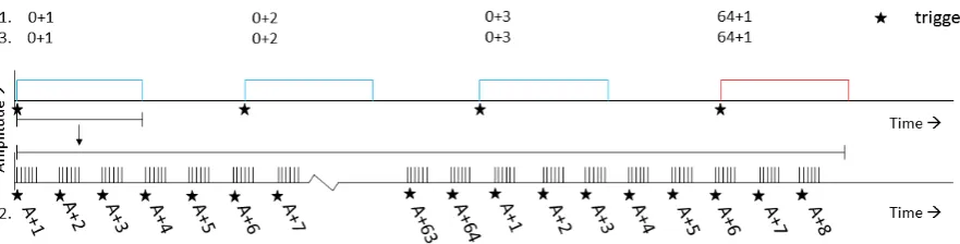
The first method is good for timing, since all timing is done by the accurate microcontroller in the stimulator. A downside of this method is that the measured EEG signal only has a trigger reference at the start of the stimulation. This would mean that it is hard to find single input signal events back from EEG measurements. Trigger codes can be set up as was done in previous experiments. Two of eight bits are used for indication of stimulation settings and six bits are used to indicate how many times a stimulus has occurred. The number of occurrence is a setting indicating how many times the stimulation with current settings has to be carried out. Figure 3.4 gives an example of trigger code generation for different experiments. The trigger codes for this experiment are calculated by equation 3.4, where TC is the trigger code, SN is the setting number and ON the occurrence number.

T C1 = 64∗SN+ON (3.4)

(20)

[image:20.595.78.519.52.164.2]

Figure 3.4: trigger codes corresponding to different experiments. Different stimulator control methods are indicated by numbers on the left. One corresponds to frequency tagging with one trigger per occurrence, two corresponds to frequency tagging with one pattern per trigger and three corresponds to tonic threshold tracking. Blue and red blocks are different signal settings. The lower axis is only used for stimulator control with one pattern per trigger and multiple triggers per stimulation. A∈[0,3].

number of patterns is passed. An overflow occurs when the fourth setting is chosen and the pattern number is 64. This trigger code can be generated as a zero, but would not result in any response of the stimulator. In this case, the overflow is escaped by writing a trigger-generating number: 1. The calculation of the trigger code can be found in equation 3.5, where PN is the number of the current pattern and the percentage sign means a modulo operation.

T C2 = 64∗SN +P N % 64 + 1 (3.5)

3.2.2 Stimulator output evaluation

The stimulator was tested and calibrated for correct output. This is done with focus on two different parts: timing and amplitude. More detailed information about the calibration process of timing can be found in appendix A. Amplitude evaluation is discussed separately since the main topics are due to the stimulator hardware instead of the controlling program. Next, a signal analysis is done in a more theoretical way to find an analytic expression for the spectrum of the stimulator output signal. The main derivation can be found in appendix B and the result will be used here. This analysis could be beneficial for later analysis of signal content of measured EEG signals.

trigger methods

(21)

[image:21.595.78.522.51.303.2]

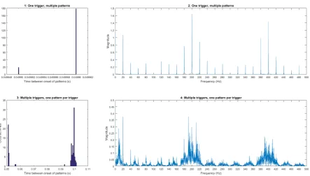
Figure 3.5: comparison of stimulus generation methods. Figures 1 and 3 are histograms of corresponding methods and figures 2 and 4 are magnitude plots of the signal in fre-quency domain.Fmod= 20Hz,P W = 1ms andIP I = 5ms.

Amplitude

The stimulator is made to generate a specific current that can be set. To measure this current, a current to voltage converter named resistor is used. The current is in the order of magnitude of several milliamps and by using a resistor of 10 KΩ, the voltage will be in the order of magnitude of 10 V. An arbitrary segment of a generated signal can be found in figure 3.6. It can be seen that the signal does not contain ideal square pulses, since there is a voltage glitch at the onset of a pulse and oscillations during the pulse. These non-ideal properties are most probably caused by the driving circuit in the stimulator. For instance parasitic capacitances in transistors could be a reason for the voltage glitch and oscillatory feedback loops could be a reason for the oscillations in the electrical current signals.

3.2.3 Signal Analysis

(22)

[image:22.595.117.486.64.238.2]

Figure 3.6: segment of stimulator output time signal over a 10 KΩresistor with 1,7 mA as specified current. Fmod= 20Hz,P W = 1ms andIP I = 5ms.

cosine. A delta function cannot exist in reality and would look like a peak with finite height and nonzero width. Due to harmonics and a pulse width that does not always have to be the same, the amplitude will be different for each peak. Frequencies at which a peak is expected can be found below, together with amplitudes (A) proportional to the harmonics.

Harmonics from IPI:A∝ 1

πn at frequencyf =nfIP I,n∈1,2,3,4, ...

Harmonics fromFmod:A∝ _πk1 at frequencyf =kfmod,k∈1,3,5,7, ...

Cross components: A∝ 1

π2_nk at frequenciesnfp±kfmod,n∈1,2,3,4, ...andk∈1,3,5,7, ...

To clarify this, magnitude information in the frequency domain of a modulated pulse train with P W = 2 ms, fmod = 13 Hz and IP I = 10 ms is plotted in figure 3.7. It can be seen that

amplitudes are highest at frequencies wherenandkare low and that amplitudes decrease for higher values ofnork. It can also be seen that peaks dependent on even multiples ofkare 0.

Figure 3.7: simulated magnitude spectrum of a modulated square wave withfmod = 13,

[image:22.595.117.479.515.676.2]

(23)

3.2.4 Threshold tracking

Threshold tracking is implemented to determine a reference for the stimulus amplitude in fre-quency tagging experiments. Threshold tracking of tonic stimuli is specifically added to the setup. To determine the tonic nociceptive threshold, the amplitude of a pulse train stimulus is increased in steps until the stimulus is felt by the subject. The amplitude is determined by using an increasing multiplier (m) multiplied by an amplitude resolution. An average threshold is adapted with each response. A response is indicated by the human subject releasing the button on the stimulator. The pulse trains with different amplitudes are separated by a spe-cifiable silent time in which a reaction of the subject is received.

The different amplitudes are generated by one trigger per pulse train corresponding to one amplitude. This is the same way as was done with frequency tagging and the one trigger and multiple patterns method. This is chosen to obtain high timing accuracy instead of many time references for EEG, since the EEG responses of threshold tracking are not intended to be used. Different trigger codes are generated per different amplitude to be able to separate pulse trains with different amplitudes in the log files. Two bits are reserved for different experiment settings, the remaining bits are used to represent the amplitude. The value of the amplitude multiplier will be used in the trigger code, as can be seen in equation 3.6. As a safety measure, the increasing amplitude cannot go beyond 2 mA.

(24)

4. Validation

A technical pilot study on one healthy human subject was performed to demonstrate and val-idate the new setup with implemented frequency tagging. Four different settings are used to stimulate the subject. First an average threshold of nociception was measured, which was used tot determine the amplitude for actual frequency tagging. The cortical activities during frequency tagging stimulation are measured with EEG. The EEG signals of electrode deriva-tions C4-Fpz, C3-Fpz and Cz-M1M2 will be analyzed to investigate potential reladeriva-tions between cortical activities and stimuli.

4.1 Materials and methods

4.1.1 Human subject

One participant (male, aged 21 years, right handed) took part in the experiment. The parti-cipant was healthy and pain-free. The partiparti-cipant did not consume any energizers or tranquil-izers (e.g. coffee or alcohol) from 24 hours before the experiment and onwards. The parti-cipant slept well the night before the experiment and had a good breakfast. The partiparti-cipant was informed by an information letter which can be found in appendix C. The experimental procedures were approved by the local ethics committee.

4.1.2 Stimuli

The subject was stimulated with modulated pulse trains. Cathodic square wave controlled current pulses of 1 ms PW, separated by 10 ms IPI, were used. The pulse train was modulated on and off with frequencies 13, 20, 33 and 43 Hz. These frequencies were chosen to measure a wide frequency band as well as prevent possible harmonics between different modulation frequencies. The stimulus amplitude was set to twice the perceptual threshold, estimated by an increasing staircase procedure of a similar modulated pulse train with a duration of 2s per amplitude to generate a definite pain sensation. IES stimulation was used to preferentially activate Aδ-fibers on the back of the left hand. The electrode consisted of five needles, based on a bimodal design [23]. A TENS electrode was used as anode and was placed on the lower arm. The electrodes were connected to the setup as described in chapter 3.

4.1.3 Procedure

(25)

to drink cold water between any of the stimuli by releasing the button on the stimulator. The subject was asked to blink as few as possible, concentrate and focus on a fixed point during the stimuli. Pulse trains with different frequency were each repeated 10 times. The total time in which stimulations were applied was approximately 30 minutes.

4.1.4 EEG measures

EEG signals were recorded using an EEG cap (ANT Neuro Waveguard) placed on the scalp. The cap contained 64 Ag/AgCl electrodes. Signals coming from the electrodes were amplified using an ANT Neuro 64-channel Refa-72 EEG amplifier and saved together with stimulus trig-ger codes on a PC. All channels were sampled with 1 kHz. All electrode impedances on the cap were kept below 5 kΩand the ground electrode was placed on the forehead.

4.1.5 Data analysis

The trigger and EEG information was analyzed using Matlab and an EEG/MEG analysis tool-box called FieldTrip. Non-overlapping EEG segments were obtained by partitioning the EEG recording relative to ten seconds before and ten seconds after all trigger times. All EEG seg-ments were filtered using a fifth order 2-480 Hz bandpass filter for removal of frequencies not relevant for this experiment and anti aliasing. Fifth order bandstop filters with center frequen-cies 50, 150, 250 and 350 Hz were used on all segments as well to remove components from the electrical grid. Eye blinking artifacts were not removed from any trials.

For each EEG segment, channel derivations C4-Fpz, C3-Fpz and Cz-M1M2 were derived. The first two channel derivations were chosen to take a bigger dipole moment into account relative to C4-Fz and C3-Fz in literature. Segments were processed in two ways per setting. First, the average of all individual segments was taken and the result was transformed using a wavelet transform. This sequence corresponds to a phase locked analysis. The wavelet transform will be tapered based on multiplication in the frequency domain and relative baseline correction is used for plotting. Second, the time during stimulus in each segment is processed. This was done by first averaging the time signals and subsequently applying a FFT transform (phase locked analysis) and by first FFT transforming each individual signal and subsequently averaging the magnitude spectrum (non phase locked analysis). Averaged signals in the fre-quency domain obtained via both methods are subsequently averaged relative to neighboring frequencies. The average of each frequency in±1 Hz around the center frequency was sub-tracted for each possible frequency in the spectrum.

(26)

4.2 Results

Results of frequency tagging with different modulation frequencies, 13, 20, 33 and 43 Hz, can respectively be found in figures 4.1, 4.2, 4.3 and 4.4. Different plots are made: one for the time signals around stimulus onset, time-frequency plots for a global overview of all data in time and frequency domain and magnitude spectrum plots in the frequency domain to have a clearer view of frequency content during stimulation. Channel derivations C4-Fpz, C3-Fpz and Cz-M1M2 are analyzed separate and are represented per column. All measurement data was based on 10 trials.

From the time signal plots around stimulus onset it can be seen that for the channel derivations C4-Fpz and C3-Fpz there are differences between before and after stimulus onset. After stim-ulus onset, it seems that there are strange components in the EEG signal, which seem similar to the stimulus pulse train. From the time plot of channel Cz-M1M2 for all different modulation frequencies, it can be seen that a phasic response is present after stimulus onset. This may be an event related potential called P300, corresponding to cognitive processing.

From the time frequency plots, it can be seen which frequencies are present at which time. For all different modulation frequencies, it can be seen that distinctive frequencies correspond-ing to multiples of the modulation frequency, multiples of the frequency correspondcorrespond-ing to the IPI of 10 ms and combinations of both multiples are present. The magnitude of these fre-quencies seems to be less in channel derivation Cz-M1M2. For segments corresponding to measurements of a modulation frequency of 20 Hz, it can be seen that there is much activity at frequencies spread around the spectrum. This is most probably due to noise from eye blinking artifacts in the recordings.

In the third row of figures with data, the magnitude with subtracted relative average can be seen. This is analyzed in both phase locked and non phase locked methods. Considering all data from all modulation frequencies, it can be said that peaks occur at combinations of mul-tiples of the modulation frequency or mulmul-tiples of the frequency corresponding to 10 ms IPI. These are frequencies that can be derived from the frequencies present in the input signal as analyzed in section 3.2.2. Proportionality of peak amplitude seems to coincide with expecta-tions most of the times. At each peak, both phase locked and non phase locked components are present and in most cases the non phase locked components have higher magnitude. This means that responses cannot be categorized as one of the two types.

For the modulation frequency of 13 Hz, it can be seen that distinct peaks are not present under 87 Hz. If the higher frequencies are considered, the highest peaks occur at the frequen-cies corresponding to the IPI. Frequency peaks at a distance of multiples of 13 hz from this can be found back in the whole spectrum. At the higher half of frequencies, multiple peaks with relatively low amplitudes are found. These correspond to combinations of higher harmonics of the modulation frequency and frequencies corresponding to the IPI.

If pulses modulated with 20 Hz are considered, it can be seen that most of the spectral peaks are again at the higher frequencies. In this case, peaks at 80 Hz and higher are distinct. If the spectrum of channel derivation C4-Fpz is looked more closely, a small peak is present at 20 Hz. If the spectrum of channel derivation C3-Fpz is looked more closely, peaks at 20, 40 and 60 Hz are present. These peaks are barely distinct, but still specific at a multiple of the modulation frequency.

(27)

non phase locked is relatively high. As frequency increases, this ratio decreases.

Results corresponding to a modulation frequency of 43 Hz seem to be quite similar to results of 33 Hz. Channel derivations C4-Fpz and C3-Fpz show harmonics with a higher amplitude than Cz-M1M2, revealing less powerful frequencies as well. Notable is that multiples of the frequency corresponding to the IPI are not present at precisely 100, 200 and 400 Hz, but at frequencies which are a multiple of the modulation frequency close by.

(28)

[image:28.595.60.781.76.474.2]

Figure 4.1: signal time plot of -0.5 to +1s relative to trigger on the first row, phase locked time-frequency analysis on the second row and frequency spectra during stimulation on the third row. Columns correspond to respective channel derivations. Data of 10 trials and a modulation frequency of 13 Hz is used.

(29)

[image:29.595.65.782.61.472.2]

(30)

[image:30.595.59.783.76.473.2]

(31)

[image:31.595.50.781.72.473.2]

(32)

[image:32.595.59.788.78.478.2]

Figure 4.5: magnitude spectrum of phase locked and non phase locked analysis of 10 trials of 50 ms before a 33 Hz stimulus onset (red) and 50 ms after stimulus onset (blue). Channel derivations C4-Fpz, C3-Fpz and Cz-M1M2 are separated respectively in each plot. Solid lines correspond to phase locked analysis (PL) and dotted lines correspond to non phase locked analysis (NPL).

(33)

5. Discussion

Outcome of this research can be interpreted in many different ways. An example is already present in the many different representation of EEG measurements in the validation experi-ment. Since these EEG recordings give the result of an experiment, this experiment can be evaluated. The implemented setup to execute this experiment can thereby very well be evalu-ated to its functional extend according to the experiment results.

5.1 Experiment

An experiment was done on a human subject in which electrical current pulses stimulated the left hand to consecutively measure EEG signals from the scalp. Stimulation was done via a pulse train that was modulated on and off with a certain frequency. EEG data from channel derivations C4-Fpz, C3-Fpz and Cz-M1M2 was analyzed.

The experiment was conducted on only one human subject. This leads to very biased results. This bias could be large, such that data that is interpreted from these measurements could lead to different conclusions than measurement data based on measurements of another hu-man subject or combinations of huhu-man subjects. Another factor making the measurements biased is the presence of eye blinking artifacts. Only 10 trials are considered, if one trial would consist of an eye blinking artifact, the time average data is already affected significantly for a specific time.

(34)

5.2 Measurement setup

A measurement setup was improved to be able to do nociceptive frequency tagging experi-ments. Main requirements of this improvement were ability to generate precisely timed pulses and a variable controlled amplitude. During calibration and tests on a human subject it was found that precise timing can be achieved by the setup. Different ways of controlling stimulator output were tested. Timing can be done correctly if it is completely managed by the micro-controller in the stimulator. A lot of jitter in timing was found when managed by a program controlling a parallel port on a desktop pc. This inaccurate timing resulted in noise and incor-rect frequency peaks in the magnitude spectrum of the signal.

(35)

6. Conclusion

The conclusion of this bachelor assignment is split up into two parts. First, conclusions about this work are drawn and second, recommendations for future research are given.

6.1 Conclusions

Increasing insight into nociceptive neural processing would lead to better understanding and treatment of increased pain sensitivity. An observation method to gain new insights is fre-quency tagging. This method uses tonic stimuli with a controlled frefre-quency content to observe corresponding nociceptive cortical information. An implementation of a setup that can be used for frequency tagging experiments was made. Results show that tonic stimuli with precise fre-quency content can be generated. Experiments with one human subject show that frequencies as a response to the input signal can be found back in EEG recordings. However, the exper-iments reveal that frequency content is available in EEG recordings in time after the stimulus onset and before cortical responses are possible. This is an indication of stimulus artifacts that are present in the EEG recordings, making measurements not interpretable for analysis of neural processing. If issues with stimulus artifacts in EEG recordings would be solved, this setup could be considered ready for frequency tagging experiments.

6.2 Recommendations

If future research is followed up on this work, the following recommendations might be taken into account:

• Two different methods were used to generate timed stimuli. The stimulator was set to generate multiple patterns if one trigger was present or the stimulator was set to gen-erate one pattern per trigger with multiple trigger signals. These two methods are com-pletely opposite to each other. A compromise could be made where multiple patterns are generated per trigger and multiple triggers are given per stimulation. This results in a tradeoff between timing accuracy and time references, since more patterns per trigger results in more timing accuracy and more triggers result in more time references in EEG recordings.

• The stimulator is programmed to accept patterns up to a certain length. If low modulation frequencies are desired, this value might have to be increased to let the stimulator work correctly.

• The validation experiment was conducted on only one human subject. To verify that a measurement setup is valid, it would be better to test on multiple human subjects. A statistical analysis could be an aid for determining the necessary amount of subjects. • Stimulus pulse trains were modulated with a certain frequency. If responses from multiple

frequencies are desired, the process of doing so could be facilitated by modulating the pulse trains with multiple frequencies at the same time instead of stimulating with different frequencies separated.

(36)

possible multiples that are the same to prevent occurrence of harmonics at the same frequency corresponding to both parameters. This keeps cause and effect separated between parameters.

• The frequency of the electrical grid (50 Hz) and corresponding odd harmonics can be found back in EEG recordings. Frequencies corresponding to chosen parameters should not coincide with these frequencies to keep a single cause for each frequency peak and to be able to apply band stop filters for frequencies corresponding to the grid without losing relevant measurement data.

• To track the cause of stimulus artifacts in EEG recordings, several different approaches could be useful. The circuit generating the stimulus in the stimulator could be analyzed and improved such that voltage glitches and oscillations are reduced. It is not certain that stimulus artifacts in EEG recordings are caused by the stimulator. A study researching not only pathways in the nervous system but also in other possible conductive path-ways between stimulus location and cortices could be done. Non-ideal stimuli from the stimulator could be modeled in this study to gain knowledge on corresponding signal processing.

(37)

7. Acknowledgments

(38)

References

[1] Dale Purves, George J. Augustine and David Fitzpatrick. Neuroscience. 2004. ISBN: 0878937250.

[2] Charles R Noback et al. The Human Nervous System, Structure and Function. 2005. ISBN: 1588290395.

[3] M.N. Baliki, P.Y. Geha and A.V. Apkarian. “Parsing pain perception between nociceptive representation and magnitude estimation”. In:Journal of Neurophysiology 2 (2009). [4] A.V. Apkarian et al. “Human brain mechanisms of pain perception and regulation in

health and disease”. In:European Journal of Pain 4 (2005).

[5] M.J. Millan. “Descending control of pain”. In:Progress in Neurobiology 6 (2002).

[6] Irene Tracey. “Nociceptive processing in the human brain”. In:Current Opinion in Neuro-biology 4 (2005).

[7] A. Mouraux, G. D. Iannetti and L. Plaghki. “Low intensity intra-epidermal electrical stim-ulation can activate Aδ-nociceptors selectively”. In:Pain150.1 (2010).

[8] L. Plaghki and A. Mouraux. “How do we selectively activate skin nociceptors with a high power infrared laser? Physiology and biophysics of laser stimulation”. In: Neurophysiolo-gie Clinique6 (2003).

[9] B. Bromm and R.D. Treede. “Nerve fibre discharges, cerebral potentials and sensations induced by CO2 laser stimulation”. In:Human Neurobiology1 (1984).

[10] A. Mouraux, E. Marot and V. Legrain. “Short trains of intra-epidermal electrical stimulation to elicit reliable behavioral and electrophysiological responses to the selective activation of nociceptors in humans”. In:Neuroscience Letters(2014).

[11] Esther M van der Heide et al. “Single pulse and pulse train modulation of cutaneous electrical stimulation: a comparison of methods.” In:Journal of clinical neurophysiology : official publication of the American Electroencephalographic Society 1 (2009).

[12] Robert J. Doll et al. “Effect of temporal stimulus properties on the nociceptive detection probability using intra-epidermal electrical stimulation”. In:Experimental Brain Research 1 (2015).

[13] Marc Schooneman. “Measurement of evoked potentials during multiple threshold track-ing of nociceptive electrocutaneous stimuli”. In: ().

[14] Nihan Alp et al. “Frequency tagging yields an objective neural signature of Gestalt form-ation”. In:Brain and Cognition(2016).

[15] E. Colon, V. Legrain and A. Mouraux. “EEG frequency tagging to dissociate the cortical responses to nociceptive and nonnociceptive stimuli”. In: Journal of cognitive neuros-cience10 (2014).

[16] Athanasia Moungou, Jean-Louis Thonnard and Andr ´e Mouraux. “EEG frequency tagging to explore the cortical activity related to the tactile exploration of natural textures”. In: Scientific Reports(2016).

[17] Elisabeth Colon et al. “Steady-state evoked potentials to tag specific components of nociceptive cortical processing”. In:NeuroImage1 (2012).

[18] Alexey M Ivanitsky et al. “Electroencephalography”. In: Encyclopedia of Neuroscience (2009).

[19] David Cohen and B. Neil Cuffin. “Demonstration of useful differences between magne-toencephalogram and electroencephalogram”. In: Electroencephalography and Clinical Neurophysiology 1 (1983).

(39)

[21] Aapo Hyv ¨arinen and Erkki Oja. “Independent Component Analysis: Algorithms and Ap-plications”. In:Analysis1 (2004).

[22] Robert J Doll et al. “Tracking of nociceptive thresholds using adaptive psychophysical methods.” In:Behavior Research Methods 1 (2014).

[23] P. Steenbergen et al. “Characterization of a bimodal electrocutaneous stimulation device”. In:IFMBE Proceedings(2008).

[24] Ryusuke Kakigi et al. “Cerebral responses following stimulation of unmyelinated C-fibers in humans: Electro- and magneto-encephalographic study”. In:Neuroscience Research 3 (2003).

(40)

A. Stimulator output calibration

The output of the stimulator is tested objectively by an oscilloscope to see if the stimulator out-put corresponds to intended stimulations. It is intended to stimulate with precise frequency ac-curacy to be certain that EEG measurement data can be related to the stimulation. Two meth-ods of stimulus generation are tested, the first one is with one trigger and multiple patterns and the second one is with multiple triggers and one pattern per trigger, as described in section 3.2. For each method a pulse train specified by parameters in table A.1 is generated. This pulse train will be stimulated by the stimulator to a 10 kΩ resistor. Parallel to this resistor is a 10 MΩinput resistance of a Tektronix MSO3014 Oscilloscope. This oscilloscope will sample it’s input signal with106 samples per 10 seconds, resulting in a measurement timing accuracy of 10µs. The waveform present at the oscilloscope is saved to a CSV file, which is used for later analysis on a PC.

Setting Value

Modulation frequency 20 Hz Stimulation time 10 s

Amplitude 1,7 mA

PW 1 ms

[image:40.595.213.383.311.396.2]

IPI 5 ms

Table A.1: settings for stimulus testing.

The raw measurement data is processed by a Matlab script. First, peak detection is used to select the start time of all pulses. This is done by checking if a sample is lower than 8 V and the next sample is higher than 8 V. After peak detection, the first pulse of a pattern is detected by checking if the time between two consecutive pulses is greater than 35% of the time it takes to perform one pattern. This number is chosen by realizing that pulses can only occur in the first 50% of a pattern and taking a margin because timing between patterns could not be precise. After obtaining the start times of all patterns, the difference between start times is calculated and plotted in a histogram. Time differences higher than 1 s were assumed to be from two different pulse trains and were therefore excluded. Raw measurement data is also processed to generate a magnitude plot of the signal in frequency domain by applying a FFT transform. This plot can be used to see if signal content is at the desired frequency. Some values in the raw data were set to infinity, these values were set to zero in order to enable correct FFT transform calculations.

(41)

[image:41.595.68.523.98.220.2] [image:41.595.80.517.349.461.2]

Figure A.1: histograms of left: one trigger and multiple patterns, right: multiple triggers, one pattern per trigger. Intended period is 0.05 s.

Figure A.2: magnitude information in frequency domain of a 20 Hz stimulus signal gen-erated by one trigger and multiple output patterns.

[image:41.595.82.520.585.703.2]

(42)

Figure A.2 and A.3 show the magnitude plot in frequency domain of the different stimulus gen-eration methods. It can be seen that the most important peak, around 20 Hz, is not at 20 Hz in figure A.3. This is due to the offset that was already observed from the histograms. In figure A.2 a very strong component around 200 Hz is present. This corresponds to the frequency representation of single pulses of 5 ms IPI. In figure A.3 it can be seen that 200 Hz peak is not a distinct peak but a frequency band with a lot of noisy amplitudes. It is assumed that this is a consequence of the widespread timing variations between consecutive patterns, also known as jitter. Apparently this jitter has more effect on higher than on lower frequencies, since the peak at 16.5 Hz is still very distinct.

To improve the timing performance of both methods, timing offsets have to be removed. Offset can be removed by reducing the IPI of the last pulse in a pattern, however the signals gener-ated by one trigger and multiple patterns are at the right frequency so this is not needed. The method of multiple triggers and one pattern per trigger needs further improvement which will be done by reducing the wait time between triggers. Figure A.3 shows a clear peak at 16.5 Hz. This corresponds with a period of 60.606 ms. To change the frequency of multiple triggers and one pattern per trigger to 20 Hz, the wait time between triggers has to be reduced with: 60.606−50 = 10.606ms. Labview only supports timing with an accuracy of milliseconds, so 11 ms will be used.

To see if removing timing offsets helps, the calculated offset was subtracted from the wait-ing time. Another measurement with the same settwait-ings as before, mentioned in table A.1, was executed. Results can be found in the histogram in figure A.4 and in the magnitude plot in fig-ure A.5. From figfig-ure A.4 it can be seen that the time differences between pattern onset are still quite different values, one value is quite close to the intended period of 0.05 s. The second one is present at double the intended frequency. From figure A.5 it can be seen that the intended frequency is represented by a sharp peak. This is good, however high peaks occur in neigh-boring frequencies as well, which are a result of periodic repetition of periodic unequal waiting times between onset of patterns. It was found that performance was not improved by choosing other constants to change waiting time of pattern generation. Two Labview functions were tried as different implementation, but both ’wait (ms)’ and ’wait until next ms multiple’ functions did not attenuate peaks at unintended frequencies.

(43)

[image:43.595.178.414.70.263.2] [image:43.595.78.519.326.435.2]

Figure A.4: histogram of multiple triggers, one pattern per trigger without offset. Intended period is 0.05 s.

Figure A.5: magnitude information in frequency domain of a 20 Hz stimulus signal gen-erated by multiple triggers and one pattern per trigger.

[image:43.595.75.528.494.743.2]

(44)

B. Fourier series analysis

Using Fourier series, a function which satisfies the Dirichlet conditions can be represented as a sum of multiple sine and cosine with different frequencies. Such analysis would be beneficial to give an analytical expression to a signal which is otherwise hard to transform to the frequency domain using Laplace or Fourier transforms, since cosine and sine have an easy to work with frequency domain representation.

The Fourier transform is calculated by:f(t) =a0+ ∞

X

n=1

ancos(2πnf0t) +bnsin(2pinf0t)

with: a0= _T1

Rt0+T t0 f(t)dt

an= _T2

Rt0+T

t0 f(t)cos(2πnf0t)dt

bn= _T2

Rt0+T

t0 f(t)sin(2πnf0t)dt

Fourier series of a block wave

An infinitely periodic square wave signal is considered (Figure B.1): x(t) =

[image:44.595.168.431.473.567.2]

if0≤t≤W 1 ifW < t < T 0 withx(t) =x(t±nT), n∈_Z

Figure B.1: square wave signal with amplitude 1, pulsewidth W and period T. From this signal the coefficients of the Fourier series can be calculated.

a0= _T1

Rt0+T

t0 f(t)dt=

1

T

RW

0 1dt= 1

T[t]W0 = WT

an= _T2

Rt0+T

t0 f(t)cos(2πnf0t)dt=

2

T

RW

0 1cos(2πnf0t)dt= 2

T

₁

2πnf0sin(2πnf0t)

W

0 =

= _πnf1

0T

sin(2πnf0W)−sin(0)

= _πn1 sin(2πnf0W)

In the special case whereW = T₂, this results in: an=sin(πn) = 0.

bn= _T2

Rt0+T

t0 f(t)sin(2πnf0t)dt=

2

T

RW

0 1sin(2πnf0t)dt= 2

T

₋₁

2πnf0cos(2πnf0t)

W

(45)

= _πnf−1

0T

cos(2πnf0W)−cos(0)

= 1−cos(2πnf0W) πn

In the special case whereW = T₂, this results in: an= 1−cos_πn(πn), which is for0for evennand

2

πn for oddn.

The coefficients result in a Fourier series of signalx(t)which is expressed as: x(t) = W_T +

∞

X

n=1

1

πnsin(2πnf0W)cos(2πnf0t) +

1−cos(2πnf0W)

πn sin(2πnf0t)

=

x(t) = W_T +

∞

X

n=1

1

πnsin(2πnf0W)cos(2πnf0t)− 1

πncos(2πnf0W)sin(2πnf0t) + 1

πnsin(2πnf0t)

Using the trigonometric angle sum identity sin(a±b) = sin(a)cos(b)±cos(a)sin(b),x(t) can be rewritten:

x(t) = W_T +

∞

X

n=1

1

πnsin(2πnf0(W −t)) + 1

πnsin(2πnf0t)

In the casew= T₂, the expression reduces to: x(t) = 1₂+

∞

X

n=1

1

πnsin(2πnf0 T

2)cos(2πnf0t)− 1

πncos(2πnf0 T

2)sin(2πnf0t) + 1

πnsin(2πnf0t)

x(t) = 1₂+

∞

X

n=1

1

πnsin(πn)cos(2πnf0t)− 1

πncos(πnf0)sin(2πnf0t) + 1

πnsin(2πnf0t)

x(t) = 1₂+

∞

X

n=1

− 1

πncos(πnf0)sin(2πnf0t) + 1

πnsin(2πnf0t)

This expression can be separated forneven or odd. For even multiples ofn: x(t) = 1₂+

∞

X

n=2,4,...

− 1

πnsin(2πnf0t) + 1

πnsin(2πnf0t)

= 1 2

and for odd multiples ofn: x(t) = 1₂+

∞

X

n=1,3,...

1

πnsin(2πnf0t) + 1

πnsin(2πnf0t)

= 1 2+ ∞ X n=1 2

πnsin(2πnf0t)

Derivation of modulated pulse train

A derivation for the Fourier series of a square wave with arbitrary duty cycle and a 50% duty cycle have been made. These will be used to express a modulated pulse train. The pulse train could be described as an infinitely long square wave with a small duty cycle. The modulation of this signal could be done by multiplying the signal with a 50% duty cycle square wave of infinite length with a lower frequency. To be consistent, this only works in the case where the frequency of the modulating wave is an integer multiple of the frequency of the pulses. In other cases, phase shifts will occur and some pulses will be smaller than others.

The pulse train is described by signalxp, the modulation block wave is described byxm and

the modulated pulse train is described byxmp, where:

xp(t) = W_T_p +

∞

X

n=1

1

πnsin(2πnfp(W −t)) + 1

πnsin(2πnfpt)

Frequency tagging of electrocutaneous stimuli for observation of cortical nociceptive processing