ISSN: 1821-1291, URL: http://www.bmathaa.org Volume 9 Issue 1(2017), Pages 31-40.
ANALYTIC STUDY OF ALLEN-CAHN EQUATION OF FRACTIONAL ORDER
DEVENDRA KUMAR, JAGDEV SINGH, DUMITRU BALEANU
Abstract. The key purpose of the present article is to analyze the
Allen-Cahn equation of fractional order. The fractional Allen-Allen-Cahn equation models the process of phase separation in iron alloys, along with order-disorder transi-tions. The analytical technique is employed to investigate the fractional model of Allen-Cahn equation. The numerical results are shown graphically. The out-comes show that the analytical technique is very efficient and user friendly for handling nonlinear fractional differential equations describing the real world problems.
1. Introduction
The Allen–Cahn (A-C) equation finds its applications in science and engineering [1-3]. The A-C equations is a nonlinear PDE expressed in the following manner
ρη(ζ, η)−ρζζ+ρ3−ρ= 0, (1.1)
with the initial condition
ρ(ζ,0) =f(ζ), (1.2)
occurs as a model to investigate the process of phase separation in iron alloys, along with order-disorder transitions. Fractional ordered derivatives supply an ex-cellent instrument for the interpretation of long memory and hereditary properties of various materials, systems and processes. It is in this sense that the key char-acteristic of positive real-order derivative, is the well known memory effect. Many real word problems demonstrate long memory properties. It has been shown by many researchers that fractional generalizations of integer order models describe the natural phenomena in a very efficient manner such as Caputo [4], Podlubny [19], Miller and Ross [16], Kilbas et al. [9], Srivastava [21], Yang et al. [23-26], Ku-mar et al. [10], Cattani et al. [5], Zhukovsky and Srivastava [27,28], Mokhtary [17] and others. Due to this reason in this work, we analyze the fractional generalization of A–C equation (1.1) presented as
2010Mathematics Subject Classification. 34A08, 35A20, 35A22.
Key words and phrases. Fractional Allen-Cahn equation; Homotopy analysis method; Laplace transform; Homotopy polynomials.
c
⃝2017 Universiteti i Prishtin¨es, Prishtin¨e, Kosov¨e. Submitted December 8, 2016. Published January 2, 2017. Communicated by H.M.Srivastava.
Dβηρ(ζ, η)−ρζζ+ρ3−ρ= 0, (1.3)
with the initial condition
ρ(ζ,0) =f(ζ), (1.4)
In Eq. (1.3)Dβηρ(ζ, η) represents the fractional order differential coefficient of the functionρ(ζ, η) in terms of Caputo. If we take β= 1,the fractional A-C equation (1.3) becomes the standard A-C equation. The nonlinear differential equations associated with fractional derivative are very hard to solve and and take a lot of time. The fractional A-C equation was studied by using homotopy analysis scheme [6]. The Chinese researcher Liao [13-15] has discovered an analytical approach named homotopy analysis method (HAM) for solving nonlinear models of physical problems. In recent times, analytical approaches have also been combined with well known Laplace transform scheme to investigate nonlinear equations by many authors such as Khuri [8], Kumar et al. [11,12], Khan [7], Swroop et al. [22], Singh et al. [20], and many others.
In the present investigation, we analyze the nonlinear fractional A-C equation with the aid of homotopy analysis transform method (HATM). The HATM is a novel and efficient amalgamation of the HAM, homotopy polynomials and standard Laplace transform scheme. It is very interesting to notice that the technique is a combi-nation of two robust computational techniques for handling nonlinear fractional problems.
2. Basic Definitions of fractional calculus and Laplace transform
Here we mention some important definitions and formulas of theory of fractional derivatives and integrals which shall be employed in this article:
Definition 1. The fractional integral operator of order β > 0, of a function
ρ(ζ, η)∈Cµ, µ≥ −1 in terms of Riemann-Liouville is expressed as [19]:
Jβρ(ζ, η) = 1 Γ(β)
∫ η
0
(η−τ)β−1ρ(ζ, τ)dτ, (β >0), (2.1)
J0ρ(ζ, η) =ρ(ζ, η). (2.2)
The following result holds for the Riemann-Liouville fractional integral:
Jβηγ = Γ(γ+ 1) Γ(γ+β+ 1)η
β+γ. (2.3)
Definition 2. The fractional derivative ofρ(ζ, η) in terms of Caputo is presented as [4]:
Dβρ(ζ, η) =Jn−βDnρ(ζ, η)
= 1
Γ(n−β) ∫ η
0
(η−τ)n−β−1ρ(n)(ζ, τ)dτ, (2.4)
forn−1< β≤n, n∈N, η >0.
L [Dβρ(ζ, η)] = pβL[ρ(ζ, η)]− n−1
∑
r=0
pβ−r−1ρ(r)(ζ,0 + ),(n −1 < β ≤ n). (2.5)
3. Basic idea of HATM
The HATM is an innovative mixture of the Laplace transform algorithm, HAM and homotopy polynomails. We take the following fractional nonlinear PDE:
Dβηρ(ζ, η) +R ρ(ζ, η) +N ρ(ζ, η) =g(ζ, η), n−1< β≤n, (3.1)
here ρ(ζ, η) indicates an unknown function of two variables ζ and η, Dβη = ∂ β ∂ηβ
represents the fractional operator of orderβ defined by Caputo,n∈N, Rdenotes the linear operator,N stands for the nonlinear part which may consist of the space derivatives of integer order or fractional order and the termg(ζ, η)denotes the source function.
Firstly, we apply the Laplace transform on fractional equation (3.1), it gives the result
L[ρ(ζ, η)]− 1
pβ n−1
∑
k=0
pβ−k−1ρ(k)(ζ,0) + 1
pβL[R ρ(ζ, η) +N ρ(ζ, η)−g(ζ, η)] = 0.
(3.2) We define the nonlinear operator in the following form
N[δ(ζ, η;q)] =L[δ(ζ, η;q)]− 1
pβ n−1
∑
k=0
pβ−k−1δ(ζ, η;q)(k)(0)
+ 1
pβL[Rδ(ζ, η;q) +N δ(ζ, η;q)−g(ζ, η)]. (3.3) In the above expression q ∈ [0,1] is representing the embedding parameter and
δ(ζ, η;q) is indicating a function depends onζ, η andq. By using the HAM [13-15], we build up a homotopy in the following manner
(1−q)L[δ(ζ, η;q)−ρ0(ζ, η)] =~qW(ζ, η)N[δ(ζ, η;q)], (3.4)
In the above equation L stands for the standard Laplace transform operator,W(ζ, η) represents a nonzero auxiliary function, ~ ̸= 0 indicates an auxiliary parameter,
ρ0(ζ, η) denotes an initial guess ofρ(ζ, η). On settingq= 0 andq= 1,it gives the results:
δ(ζ, η; 0) =ρ0(ζ, η), δ(ζ, η; 1) =ρ(ζ, η), (3.5)
respectively. It is obvious that as the values of q increases from 0 to 1, the solution
δ(ζ, η;q) changes from the initial guessρ0(ζ, η) to the solutionρ(ζ, η).On express-ingδ(ζ, η;q) in series form with respect toqby using well known Taylor’s theorem, we have
δ(ζ, η;q) =ρ0(ζ, η) + ∞ ∑
m=1
ρm(ζ, η)qm, (3.6)
ρm(ζ, η) = 1
m!
∂mδ(ζ, η;q)
∂qm |q=0. (3.7)
If ~ and W(ζ, η) are selected in proper way, the series (3.6) converges at q = 1, then we have
ρ(ζ, η) =ρ0(ζ, η) +
∞ ∑
m=1
ρm(ζ, η). (3.8)
The Eq. (3.8) must be one of the solutions of the nonlinear fractional equation (3.1). Now, we differentiate the Eq. (3.4) m-times with respect to q and then the resulting expression is divided by m! and finally letting q = 0, we arrive at the subsequent equation:
L[ρm(ζ, η)−χmρm−1(ζ, η)] =~W(ζ, η)ℜm(⃗ρm−1). (3.9)
Now using the inverse of Laplace transform operator on Eq. (3.9), we have
ρm(ζ, η) =χmρm−1(ζ, η) +~L−1[W(ζ, η)ℜm(⃗ρm−1)]. (3.10)
where
ℜm(⃗ρm−1) =L[ρm−1(ζ, η)]−(1−χm) 1
pβ n∑−1
k=0
pβ−k−1δ(ζ, η;q)(k)(0)
+ 1
pβ[Lρm−1+Bm−1−g(ζ, η)], (3.11)
χm=
{
0, m≤1,
1, m >1 (3.12)
Bm(ρ0, ρ1, ..., ρm) are homotopy polynomials [18] given in the following form
Bm= 1 Γ(m)
[
∂m
∂qmN δ(ζ, η;q)
]
q=0
, (3.13)
and
δ(ζ, η;q) =δ0+qδ1+q2δ2+· · · . (3.14)
4. HATM for nonlinear fractional Allen-Cahn equation
Firstly, we apply the Laplace transform on fractional A-C equation (1.3) and use the initial condition (1.4), it gives the result
L[ρ(ζ, η)]−1
pf(ζ) +
1
pβL
[
−ρζζ+ρ3−ρ
]
= 0. (4.1)
We define the nonlinear operator in the following form
N[δ(ζ, η;q)] =L[δ(ζ, η;q)]]−1
pf(ζ) +
1
pβL
[
−δζζ(ζ, η;q) +δ3(ζ, η;q)−δ(ζ, η;q)
]
.
(4.2) The mth-order deformation equation is presented as:
L[ρm(ζ, η)−χmρm−1(ζ, η)] =~W(ζ, η)ℜm(⃗ρm−1). (4.3)
ρm(ζ, η) =χmρm−1(ζ, η) +~L−1[W(ζ, η)ℜm(⃗ρm−1)]. (4.4)
where
ℜm(ρ⃗m−1) =L[ρm−1(ζ, η)]−(1−χm) f(ζ)
p +
1
pβ
[
−∂2ρm−1
∂ζ2 +Bm−1−ρm−1
]
,
(4.5)
χm=
{
0, m≤1,
1, m >1 (4.6)
Bm(ρ0, ρ1, ..., ρm) are homotopy polynomials [18] given in the following form
Bm= 1 Γ(m)
[
∂m ∂qmδ
3(ζ, η;q)
]
q=0
, (4.7)
and
δ(ζ, η;q) =δ0+qδ1+q2δ2+· · · . (4.8)
Next, on taking the initial approximationρ0(ζ, η) =f(ζ), W(ζ, η) = 1 and using the recursive relation (4.4), we have the following iterates of the HATM solution:
ρ1(ζ, η) =~
[
−f′′(ζ) +f3(ζ)−f(ζ) ] ηβ
Γ(β+ 1), (4.9)
ρ2(ζ, η) =~(1 +~)
[
−f′′(ζ) +f3(ζ)−f(ζ) ] ηβ
Γ(β+ 1)
+~2[f′′′′(ζ)−6f(ζ)(f′)2(ζ)−6f2(ζ)f′(ζ) + 3f2(ζ)−4f3(ζ)
+ 2f′′(ζ) +f(ζ)] η
2β
Γ(2β+ 1) (4.10)
.. .
Making use of the same process, the componentsρm, m≥0 of the HATM solution can be found and consequently the solution completely obtained.
Hence, we approximate the HATM solution by the truncated series
ρ(ζ, η) = lim N→∞
N
∑
m=0
ρm(ζ, η). (4.11)
5. Numerical results and discussions
We calculate the numerical results for different values of space variable ζ, time variable η and time-fractional Brownian motions β = 0.75, 0.50, 0.25 and for the standard motionβ = 1. In order to compute numerical results, we take the initial conditionρ(ζ,0) =f(ζ) = 1
1+exp(−√2 2 ζ
) for nonlinear fractional AC equation (1.3).
The numerical results for the distanceρ(ζ, η) for different values of space variable
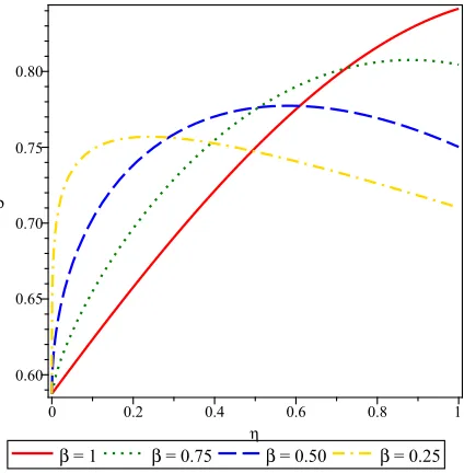
ζ, time variable η and β are depicted through Figs. 1-6. Fig. 1 represents the
Figure 1. ~−curve of HATM solution for various responses ofβ
atζ= 1 andη= 0.1.
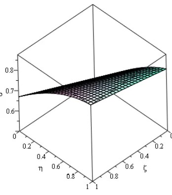
Figure 2. The surface of the HATM solutionρ(ζ, η) w.r.t. ζand
η are found, whenβ= 1 andh=−1.
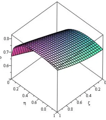
Figure 3. The response of the HATM solution ρ(ζ, η) w.r.t. ζ andη are found, whenβ= 0.75 andh=−1.
Figure 4. The response of the HATM solution ρ(ζ, η) w.r.t. ζ andη are found, whenβ= 0.50 andh=−1.
Figure 5. The response of the HATM solution ρ(ζ, η) w.r.t. ζ andη are found, whenβ= 0.25 andh=−1.
6. Conclusions
In this study, the fractional A-C equation is successfully examined with the aid of HATM. The HATM is a very innovative and strong computational approach to solve nonlinear fractional equations. The HATM contains an auxiliary parameter
~ by which we can insure the convergence of the solutions. Thus, it to be worth mentioning that the HATM is very simple, easy to use and more powerful com-putational scheme for analyzing nonlinear problems. The most important part of this investigation is to analyze the fractional A-C equation and related issues. The numerical results for distanceρ(ζ, η) are presented graphically that reveals that the order of derivative significantly affects the distance. Hence, it is to be concluded that the proposed algorithm is very powerful and well organized to study analyt-ically as well as numeranalyt-ically to fractional order mathematical models describe the real world problems in a better and systematic manner.
Acknowledgments. The authors would like to thank the anonymous referees for their comments and suggestions that helped us to improve this paper.
References
[1] S. M. Allen and J. W. Cahn,On tricritical points resulting from the intersection of lines of higher-ordered transitions with spinodals, Scr. Metall.10(1976) 451-454.
[2] L. Bronsard and F. Reitich, On three-phase boundary motion and the singular limit of a vector valued Ginzburg-Landau equation, Arch. Rat. Mech. Anal.124 (1993) 355-379. [3] J. W. Cahn and S. M. Allen,A microscopic theory of domain wall motion and its experimental
verification in Fe-Al alloy domain growth kinetics, J. Phys.38 (1977) 47-51. [4] M. Caputo,Elasticita e Dissipazione, Zani-Chelli, Bologna, 1969.
[5] C. Cattani, H. M. Srivastava and X.-J. Yang (Editors), Fractional Dynamics, Emerging Science Publishers (De Gruyter Open), Berlin and Warsaw, 2015.
[6] A. Esen, N. M. Yagmurlu and O. Tasbozan, Approximate Analytical Solution to Time-Fractional Damped Burger and Cahn- Allen Equations, Appl. Math. Inf. Sci. 7 5 (2013) 1951-1956.
[7] M. Khan M. A. Gondal, I. Hussain and S. K. Vanani, A new comparative study between homotopy analysis transform method and homotopy perturbation transform method on semi infinite domain, Math. Comput. Model.55(2012) 1143-1150.
[8] S. A. Khuri, A Laplace decomposition algorithm applied to a class of nonlinear differential equations, J. Appl. Math.1 (2001), 141-155.
[9] A. A. Kilbas, H. M. Srivastava and J.J. Trujillo, Theory and Applications of Fractional Differential Equations, North-Holland athematics Studies, vol. 204, Elsevier, Amsterdam, 2006.
[10] D. Kumar, J. Singh and D. Baleanu, Numerical computation of a fractional model of differential-difference equation J. Comput. Nonl. Dyn.11(2016), doi: 10.1115/1.4033899. [11] D. Kumar, J. Singh and S. Kumar, A fractional model of Navier-Stokes equation arising in
unsteady flow of a viscous fluidJournal of the Association of Arab Universities for Basic and Applied Sciences17(2015) 14-19
[12] D. Kumar, J. Singh and S. Kumar, Numerical computation of nonlinear fractional Zakharov-Kuznetsov equation arising in ion-acoustic waves, J. Egyptian Math. Soc.22(2014) 373-378. [13] S. J. LiaoBeyond Perturbation: Introduction to Homotopy Analysis Method, Chapman and
Hall / CRC Press, Boca Raton, 2003.
[14] S. J. Liao An approximate solution technique not depending on small parameters: a special example, Int. J. Nonlinear Mech.30(1995) 371-380.
[15] S. J. Liao Homotopy analysis method in nonlinear differential equations, Springer and Higher Education Press, Berlin and Beijing, 2012.
[17] P. Mokhtary, F. Ghoreishi and H. M. Srivastava,The Mu¨ntz-Legendre Tau method for frac-tional differential equations, Appl. Math. Modelling40(2016), 671-684.
[18] Z. Odibat and S. A. Bataineh, An adaptation of homotopy analysis method for reliable treat-ment of strongly nonlinear problems: construction of homotopy polynomials, Math. Meth. Appl. Sci. (2014), doi: 10.1002/mma.3136.
[19] I. Podlubny,Fractional Differential Equations, Academic Press, New York, 1999.
[20] J. Singh, D. Kumar and R. Swroop, Numerical solution of time- and space-fractional coupled Burgers equations via homotopy algorithm, Alexandria Eng. J.55 2(2016), 1753-1763. [21] H. M. Srivastava,Some families of Mittag-Leffler type functions and associated operators of
fractional calculus, TWMS J. Pure Appl. Math.7(2016), 123-145.
[22] R. Swroop, J. Singh and D. Kumar,Numerical study for time-fractional Schr¨0dinger equa-tions arising in quantum mechanics, Nonlinear Eng.3 3(2014) 169-177.
[23] X.-J. Yang, D. Baleanu, and H. M. Srivastava, Local Fractional Integral Transforms and Their Applications, Academic Press (Elsevier Science Publishers), Amsterdam, Heidelberg, London and New York, 2016.
[24] X.-J. Yang, F. Gao and H.M. Srivastava, Exact travelling wave solutions for the local fractional two-dimensional Burgers-type equations, Comput. Math. Appl. (2016), http://dx.doi.org/10.1016/j.camwa.2016.11.012.
[25] X.-J. Yang, J. A. T. Machado and H. M. Srivastava,A new numerical technique for solv-ing the local fractional diffusion equation: Two-dimensional extended differential transform approach, Appl. Math. Comput.274(2016), 143-151.
[26] X.-J. Yang, Z.-Z. Zhang and H. M. Srivastava, Some new applications of heat and fluid flows via fractional derivatives without singular kernel, Thermal Sci.20(Suppl. 3) (2016), S835-S841.
[27] K. V. Zhukovsky and H. M. Srivastava,Analytical solutions for heat diffusion beyond Fourier law, Appl. Math. Comput.293(2017) 423-437.
[28] K. V. Zhukovsky and H. M. Srivastava, Operational solution of non-integer ordinary and evolution-type partial differential equations, Axioms5(2016), Article ID 29, 1-21.
Devendra Kumar
Department of Mathematics, JECRC University, Jaipur-303905, Rajasthan, India E-mail address:[email protected]
Jagdev Singh
Department of Mathematics, JECRC University, Jaipur-303905, Rajasthan, India E-mail address:[email protected]
Dumitru Baleanu
Department of Mathematics, Faculty of Arts and Sciences, Cankaya University, Eskise-hir Yolu 29. Km, Yukariyurtcu Mahallesi Mimar Sinan Caddesi No: 4 06790, Etimesgut, Turkey