Dynamic modeling of a heat exchanger

(1)

Internship at Powerspex

Dynamic modeling of a heat exchanger

Job Rutgers

s0199915

29-02-2016 - 17-06-2016

Powerspex

Department Research& Development Hengelo, the Netherlands

Supervisor Johan Schmaal

University of Twente

(2)

Preface

This report has been written during my internship at Powerspex. The internship took place at the department research and development (R&D), currently responsible for developing its own Java based simulation software PsxCad and the models within this software. The program is used to simulate Distributed Control Systems (DCS) and Supervisory Control And Data Ac-quisition (SCADA) systems. The software is applied for example training simulators for power plants. During my internship I have been part of the team which provided me insight in the work done by this department. My main assignment consisted of making another model for the heat exchanger, which does not suffer from numerical instabilities. Furthermore this internships also gave the possibility to get a impression of the training simulator for Velsen 24 & 25. I would like to thank my colleagues at R&D department. I felt really welcome and have been treated as part of their team.

Job Rutgers

(3)

Abstract

This internship has been done at Powerspex, at the department R&D, mainly responsible for the development and implementation of dynamic training simulators. These training simulators are built in a program called PsxCad, which is a Java-based program completely developed by Powerspex.

My main assignment during this internship consisted of developing a new model for a heat exchanger. The current logarithmic mean temperature difference model does not satisfy, espe-cially during startup situations. The heat capacity is not taken into account in this model and there are also numerical instabilities.

Two new models for the heat exchanger were built based on a discretized finite volume method. Both flows and the wall were divided in elements and the laws for mass and energy conservation were applied. The heat capacitance of the wall was included in the calculations as well. The first model is based on iterative calculations of the parameters, while the second model uses the values of the previous time step to calculate the temperature, enthalpy and heat exchange.

The results were generated using a demo process model , which uses three different heat counter current heat exchangers. For all three models the outcomes were plotted and the differences investigated.

The results showed that model two provided a suitable and stable outcome without losing a lot of computational power. Moreover, the included wall capacitance is visible. The disadvantage of this model is the complexity in comparison with the current model.

(4)

1 Company and department

Powerspex is a technical company specialized in energy and automation solutions, with projects in different working areas like engineering, building, testing, commissioning on site and proving service. The history of Powerspex starts in 1997 as a part of Stork. After being sold to NEM Energy Services and being part of Siemens, the company became independent in 2013. Nowadays Powerspex has about 60 employees with different levels of education.[1, 2]

1.1 R&D department

The group consist of 5 employees, with different backgrounds. The main focus of the group are the training simulators, which are mainly build to train operators of power stations. By making a virtual installation, with logic and control, process models and operator panels, it is possible to simulate different kinds of scenarios during operation. The software provides in simulating DCS, Human Machine Interface (HMI) and Programmable logic controller (PLC) systems.

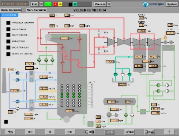
[image:5.595.117.480.408.685.2]

The R&D department is concerned with developing its own software package PsxCad, which is based on the Java platform. In the past The training simulators were built with PsxCad in combination with HCADwin. PsxCad did the operator interface (figure 1.1 shows an example), with look-a-like screens of the real operator panels. Via a web interface it was coupled with HCADwin, which was responsible for the logics and process models. For the new simulators they made the change to make both logics, process models and operator interface in PsxCad. The advantages of the new software are a small footprint, it is light weight, the possibility to run cross platform and to run on a single computer. Depending on the size of the project it possible to run the simulation multiple times faster than real-time.

(6)

2 Simulation environment

PsxCad has a kind of ’drag and drop’ environment, a bit like a flow sheeting program or Matlab Simulink, where all kinds of blocks can be connected to one another. These blocks can contain logics, controllers or a model, for example. By linking all those blocks together, a process model can be realized. In order to create the same ’look and feel’ for the operator of the simulator as for the operator of real plant, PsxCad has also a possibility to create all kind of different graphical items. With these items imitations of the operation screens and pop-ups of the installations, can be created.

2.1 Performance, stability and accuracy

Important aspects for simulation are performance, stability and accuracy. For PsxCad the performance is one of the most important issues. In case a much higher performance can be obtained by leaving aspects with less influence out of a model, this will be preferred. Usually not all the parameters of an installation are known. In order to get the behavior of the system in accordance with the real installation, the parameters will be tweaked until the system behaves like the real installation.

Stability issues are also playing a role in the simulation, because of the discrete calculations, with time steps of 0.1 second. Instability of the simulation will mainly occur during the startup phase of an installation. By initializing the model with the right initial parameters and by applying some damping and delay factors the instability can be reduced. Little instability is accepted, if it will converge within a certain time to a stable condition.

The simulator is just an approximation of a real installation, with assumptions in all the used models. However, despite these assumptions, the results of the simulator have the same order of magnitude as the real installation.

2.2 Flow- and pressure points

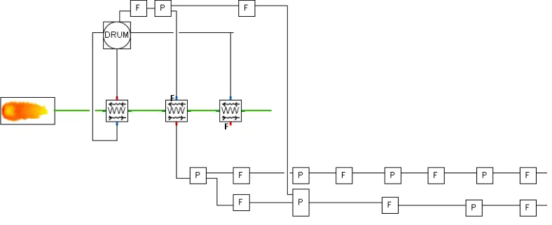
[image:6.595.103.497.567.728.2]

The process model consists of different blocks, as shown in figure 2.1. These blocks are parts of the installation, for example a pump, furnace, drum or a heat exchanger. In order to get the right mass flows and pressures between the connected blocks, flow and pressure points are introduced. Sometimes the points are already included in the blocks, and in other cases they can be drawn as separated blocks. The pressure point is an integrator which relates the pressure change of the system to the mass flow going through the pressure point. The flow point can be seen as a kind of valve, where the position of the valve, the area and the density ρ of the medium (defined by the pressure and enthalpy) are determining the mass flow.

(7)

3 Theoretical analysis of the heat exchanger

In the energy industry transfer of heat to and from process fluids is an essential part of the process. This is mainly done by heat exchangers. The definition of a heat exchanger is ’a device that is used to transfer thermal energy between two or more fluids, between a solid surface and a fluid, or between solid particles and a fluid, at differing temperatures and in thermal contact, usually without external heat and work interactions’.[3]

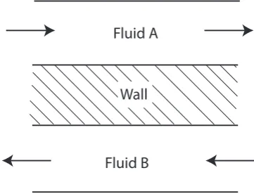
Usually a heat transfer surface separates the fluids in most of heat exchangers. The surface is in direct contact with the fluids and transfers the heat by conduction. The heat transfer between the surface and the bulk of the fluids is mainly caused by convection. The most effective way of heat transfer is through a counter current heat exchanger. In the industries there are all different types of heat exchanger designs available. For the modeling purpose of this report a simplified two fluid counter current heat exchanger is used with a one-dimensional flow, as shown in figure 3.1. [4] For the modeling of the heat exchanger the following assumptions have been made [5, 6]:

The fluid flows are simplified as a one-dimensional homogeneous flow regime.

In and out flow of mass is equal.

Axial heat conduction of the fluids can be neglected.

Infinite wall thermal conductivity (wall temperature is considered to be the same on both sides of one wall cell).

Heat flow to the ambient is negligible.

Kinetic energy of the fluids can be neglected.

Pressure drops within the heat exchanger are neglected.

Fluid A

[image:7.595.206.387.456.594.2]

Fluid B Wall

Figure 3.1: The counter current heat exchanger

3.1 Mass and energy conservation

Based on the above assumptions, the equations of conservation for mass and energy can be expressed as follows [5, 7]:

∂ρ ∂t +

∂(ρu)

∂x = 0 (3.1)

∂(ρh−P)

∂t +

∂(ρhu)

∂x =k

∂2T

(8)

Since the assumption is made that the pressure drop is negligible, the momentum-conservation equation vanishes.

For simulation purposes the equations are expressed in terms of mass flow rate, by multiplying with the cross-sectional area Acr.

∂ρAcr

∂t +

∂m˙

∂x = 0 (3.3)

∂(ρhAcr−P Acr)

∂t +

∂( ˙mh)

∂x =Acrk ∂2T

∂y2 (3.4)

By rearranging equation 3.4 and writing it as a control volume, whereVcv =Acr∆xthe equation

of energy becomes [8]:

Vcv

h∂(ρh)

∂t −

∂P ∂t

i

cv= ˙Qcv+

X

( ˙mh)in−

X

( ˙mh)out (3.5)

The equation can be simplified further by neglecting the work associated with the time rate of change of pressure.equations

Vcv

∂(ρh)cv

∂t = ˙Qcv+

X

( ˙mh)in−

X

( ˙mh)out (3.6)

The principle of conservation of mass can be written as:

Vcv

∂ρ ∂t =

X

˙

min−

X

˙

mout (3.7)

The expression can be reused by the assumption that the mass flow into and out of the control volume is equal.

Vcv

∂ρ

∂t = 0 (3.8)

This implies that when the control volume is constant the density is constant as well. Equation 3.6 can now be modified to equations:

(ρV)cv

∂hcv

∂t = ˙Qcv+

X

( ˙mh)in−

X

( ˙mh)out (3.9)

The parameter ˙Qcv denotes the heat transfer which can be written as:

˙

Qcv=A·U·(Tw−Tf) (3.10)

In this formula U [W/K/m2] the overall heat transfer coefficient and A is the contact surface between the wall and the fluid.

3.2 Conduction

The conduction of the heat through the wall depends on the temperature, the surface area, the thickness of the wall and the conductivity of the material of the wall. Because the thickness of the wall in a heat exchanger is relatively small the temperatures of the wall are considered equal on both sides. This implies that the thermal resistance of the wall can be neglected. [6] The energy balance of the wall, when considering the wall capacitance, becomes as follow:

ρV Cp

∂T

∂t −Q˙A+ ˙QB= 0 (3.11)

Where ρ, V and Cp are the density, the volume and the heat capacity coefficient of the wall

(9)

3.3 Convection

Convection mainly takes place between the bulk of the fluid and the wall, and can be calculated with ˙Qconv =A·hconv·(Tf −Tw). The flow conditions and boundary layer have an influence

on the convective heat transfer coefficient hconv. The Nusselt numberN uis characterizing this

dependency. [6]

hconv=

N u·k

D (3.12)

Where D is some characteristic length and k is the conductivity of the fluid. The Nusselt number can be calculated as a function of ReynoldsRe and PrandtlP r.

Re= ρ·v·D

µ (3.13)

P r = µ·cp

k (3.14)

Whereρ is the density of the fluid,v mean velocity of the fluid,µthe dynamic viscosity of the fluid andCp the specific heat of the fluid.

The Nusselt number can be calculated with the following relation given in literature:

N u=a·Reb·P rc (3.15)

Where a, b and c are constants which need to be selected depending on the situation, but generally are 0.023, 0.8 and 1/3 respectively.

3.4 Transient simulation

(10)

4 Model formulation

Based on the theory, two models for a heat exchanger have been built. The models are based on the simplified counter current heat exchanger, as shown in figure 3.1. The fluids which flow through the heat exchanger were water/steam and flue gas. The properties of water and steam are obtained using steam tables according to IAPWS IF-97. For the flue gas properties functions were used as described in appendix A

4.1 Current Model

The current model that is used for the heat exchanger is based on the logarithmic mean time difference (LMTD). The heat transfer areaA0 and the general heat transfer coefficient UW W,0

of the heat exchanger are set. For the initial step the temperature going in and out , enthalpy, mass flow and pressure for both sides should also be defined.

There is insufficient information known to calculate the heat transfer coefficient as described in paragraph 3.3, So the heat transfer coefficient is made dependent of one of the two mass flows scaled with a design mass flow to the power 0.6.

UW W =UW W,0·

˙

mB

˙

mdesign

0.6

(4.1)

Where UW W,0 is the specified overall heat transfer coefficient and ˙mdesign is a value which

indicates the design mass flow.

The energy change of both sides is calculated with:

˙

QA= ˙mnA·(hnA,out−1 −h n A,in)

˙

QB= ˙mnB·(hnB,in−hn

−1

B,out)

(4.2)

The enthalpy change within a time step is calculated with the energy difference between the energy of the flow and the energy transfer calculated with the LMTD divided with a predefined mass.

∆hA

∆t =

˙

Qn_{LM T D}−1 −Q˙A

M ass

∆hB

∆t =

˙

QB−Q˙nLM T D−1

M ass

(4.3)

The new enthalpy of the outflow can be calculated as follows:

hn_A,out=hn_A,out−1 +∆hA ∆t ·∆t

hn_B,out=hn_B,out−1 + ∆hB ∆t ·∆t

(4.4)

The temperatures of the outflows can now be calculated using the steam and flue gas functions with thehn_A,out and hn_B,out as input.

A check is built in to be sure theTB,out> TA,inin the caseTB,in> TA,inandTB,out<(TA,in+1).

If this is true, TB,out is set to the temperature of (TA,in+ 1) and HB,out is also changed to a

enthalpy value corresponding with this temperature.

Now the ∆T1 and ∆T2 can be determined needed for the LMTD.

∆T1 =TB,in−TA,out

∆T2 =TB,out−TA,in

(11)

In order to get a valid LMTD the difference between ∆T1 and ∆T2 should not be 0 and ∆T1

and ∆T2 should be larger than 0.0001 °C, or ∆T1 and ∆T2 should be smaller than 0. If this is

true the LMTD is calculated as follow:

LM T D= (∆T1−∆T2)

ln(∆T1

∆T2)

(4.6)

Otherwise the LM T D gets the value of ∆T1.

Now ˙Qn_{LM T D} can be calculated.

˙

Qn_{LM T D}=A·UW W·LM T D (4.7)

WhereA is the surface area between the fluid and the wall.

In this way the LMTD is transformed from a formula which can be used in steady-state calcula-tion to a form to be appied for transient simulacalcula-tion. A few checks are built in to avoid division by zero in the LMTD, but these checks could still give some instabilities. Using values of the previous time step could cause some problems as well. Furthermore this model does also not include the heat capicity of the wall.

4.2 Model 1

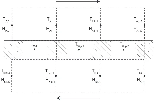
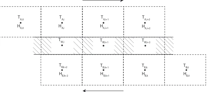
The first new model developed is based on iterative solving of the outgoing temperature and enthalpy of small discrete elements. A schematic overview of the discretized elements is shown in Figure 4.1.

T_A,i+1

H_B,k+1

T_W,j+1

H_B,k

H_B,k+2

T_A,i T_A,i+2

T_W,j+2

T_W,j

HA,i HA,i+1 HA,i+2

T_B,k+2 TB,k+1 TB,k

T_A,0

HA,0

[image:11.595.149.446.395.589.2]

H_B,0 TB,0

Figure 4.1: Discretized scheme of counter current heat exchanger model

There is a constant flow of mass in and out of each cell. The nodes with the index i = 0 and k = 0 are considered as the input flows with the enthalpy, temperature and pressure of a previous model of the simulation. And these indexes go from 0..N. The nodes of the wall, indicated with j and positioned in the middle of a fluid element, run from j = 1..N. For the nodes 1..N the following calculations have been made in each element of the flow:

UA=UA,0·

˙

mn_A

˙

mA,design

0.6

(4.8)

The heat transfer coefficientUA,0 is made dependent of the mass flow scaled with a design mass

(12)

As first estimation for the iterated solver is the temperature of the previous element that is used.

TA,i =TA,i−1 (4.9)

The heat transfer between the fluid and the wall is calculated.

˙

QA,j =UAn·

AA

N ·(TA,i−T

n−1

W,j ) (4.10)

AA is the total surface area between fluid A and the wall. Dividing by the number of elements

N it results in the surface area of the element.

By manipulating ˙Q = ˙m·∆h, an expression for the outgoing enthalpy of the element can be found:

hA,i =hA,i−1−

˙

QA,j

˙

mn_A (4.11)

The temperature can now be calculated using the steam function.

T_A,i∗ =ST EAMT(PA,i, hA,i) (4.12)

After this initial estimation the temperature can be iterated until the difference in value ofTA,i

and T_A,i∗ is smaller than 0.1 °C, with a maximum of 25 iterative steps. In this while loop the following calculations have been done:

TA,i = 0.5·(TA,i+TA,i∗ ) (4.13)

˙

QA,j =UAn·

AA

N ·(

TA,i+TA,i−1

2 −T

n−1

W,j ) (4.14)

hn_A,i =hn−1−Q˙A,j

˙

mn_A (4.15)

T_A,i∗ =ST EAMT(PA,i, hA,i) (4.16)

In case the mass flow of an element is zero, the iterative part is skipped and the outgoing temperature and enthalpy are set equal the incoming values. The heat transfer is set to zero. If the mass flow is really small, the enthalpy change of equation 4.15 becomes unrealistic large. To recude the influance of unrealistic large enthalpy values, the following conditions have been applied:

Limiting the values of the enthalpy between 40 and 3700kJ/kg.

Limiting T_A,i∗ at the wall temperature whenTA,0 < Tw,0

In case the number of iterations is larger than 10; Let the output temperature (TA,i) of

an element slowly go to the wall temperature of that element, for the subsequent steps.

(13)

UB=UB,0·

˙

mn_B

˙

mB,design

0.6

(4.17)

As first estimation for the iterated solver is the temperature of the previous element that is used.

T_B,k∗ =TB,k−1 (4.18)

The specific heat of the flue gas can be determined using the mass fraction of each component in the flue gas and the temperature.

cp,B,k−1 =F lueGascp(y, TB,k−1) (4.19)

Now a mesh number of transfer units is introduced:

∆NB,k−0.5 =

Ub·A_NB

˙

mn_B·cp,B,k−1

(4.20)

TB,k =

1

1 + 0.5·∆NB,k−0.5

·((1−0.5·∆NB,k−0.5)TB,k−1+ ∆NB,k−0.5·T_w,Nn−1₋₍_j₋₁₎ (4.21)

After this initial estimation the temperature can be iterated until the difference in value ofTB,k

and T_B,k∗ is smaller than 0.1 °C. In this while loop the following calculations are done:

T_B,k∗ =TB,k (4.22)

cp,B,k =F lueGascp(x, TB,k) (4.23)

∆NB,k−0.5 =

2·Ub·A_NB

˙

mn_B·(cp,B,k−1+cp,B,k)

(4.24)

TB,k =

1

1 + 0.5·∆NB,k−0.5

·((1−0.5·∆NB,k−0.5)TB,k−1+ ∆NB,k−0.5·T_w,Nn−1₋₍_j₋₁₎ (4.25)

In case the mass flow of an element is zero, the iterative part has been skipped and the outgoing temperature is set equal to the incoming value.

After the condition for the temperature is satisfied the outflowing enthalpy of the element and the heat transfer in the middle of the element to the wall note can be calculated.

hB,k =F lueGash(y, TB,k) (4.26)

Q_B,N−(j−1) = ˙mnB∗(hB,k−hB,k−1) (4.27)

After the heat transfer between the fluid elements and the wall is has been found, the temper-ature change of the wall can be calculated. By manipulating equation 3.11, the change in wall temperature can be found as follows:

∆T_W,jn = QA,j+QB,N−(j−1)

CP,W ·M ass_N w

(14)

T_W,jn =T_W,jn−1+ ∆T_W,jn (4.29)

Due to the iterative calculations this model needs a lot of computational power. In case the mass flows are low, the model faces problems with instabilities and fixes for unrealistic enthalpy values.

4.3 Model 2

Because the first model has some problems in case of low mass flows and also uses a lot more computational power than the current model, a second model has been developed. A schematic overview of the discretized elements is shown in Figure 4.2.[6, 10]

T

A,i+1

H

B,k+1

T_W,i+1

H

B,k

H

B,k+2

T

A,i TA,i+2

T_W,i+2 T_W,i

H_A,i H_A,i+1 H_A,i+2

T_B,k+2 T_B,k+1 T_B,k

T

A,0

H_A,0

H

B,0

[image:14.595.118.481.237.398.2]

T_B,0

Figure 4.2: Discretized scheme of counter current heat exchanger model

This model assumes that the temperature in each cell is constant and there is a constant flow of mass in and out of each cell.

The nodes with the indexi= 0 and k= 0 are considered as the input flows with the enthalpy, temperature and pressure of a previous model of the simulation. For the nodes 1..N the following calculations are made in each element of the flow:

UA=UA,0·

˙

mn_A

˙

mA,design

0.6

(4.30)

The heat transfer coefficientUA,0 is made dependent of the mass flow scaled with a design mass

flow to the power 0.6.

˙

Qn_A,i =U_An·AA

N ·(T

n−1

A,i −T

n−1

W,i ) (4.31)

AA is the total surface area between fluid A and the wall. Dividing by the number of elements

N it results in the surface area of the element.

By manipulating equation 3.9, the enthalpy change can be defined as follow:

∆hn_A,i = m˙

n A·(hn

−1

A,i−1−h

n−1

A,i )−Q˙nA,i

M assA

·∆t (4.32)

The (ρV)cv of (3.9) can be seen as a mass.

(15)

The temperature can now be calculated using the steam function.

T_A,in =ST EAMT(PA,in , hnA,i) (4.34)

The calculations of the B side of the heat exchanger are quite similar, except for the flue gas flowing through and the used wall note because of the counter flow heat exchanger.

UB=UB,0·

˙

mn_B

˙

mB,design

0.6

(4.35)

˙

Qn_B,k =U_Bn·AB

N ·(T

n−1

B,k −T

n−1

W,N−(k−1)) (4.36)

∆hn_B,k = m˙

n

B·(h

n−1

B,k−1−h

n−1

B,k)−Q˙nB,k

M assB

·∆t (4.37)

hn_B,k =hn_B,k−1+ ∆hn_B,k (4.38)

The temperature of the flue gas can be determined using the mass fraction of each component in the flue gas and the calculated enthalpy.

T_B,kn =F lueGasT(y, hnB,k) (4.39)

By manipulating equation 3.11, the change in wall temperature can be found.

∆T_W,in = Q

n

A,i+QnB,N−(i−1)

CP,W ·M ass_N w

·∆t (4.40)

T_W,in =T_W,in−1+ ∆T_W,in (4.41)

(16)

5 Results

In order to compare the results of the different heat exchanger models the process model of figure 2.1 is used. This process model was a demo model which already existed. For the three heat exchangers in this model boiler, superheater and economizer their input and output values of the heat exchangers have been measured during a time of 600 seconds.

5.1 Boiler

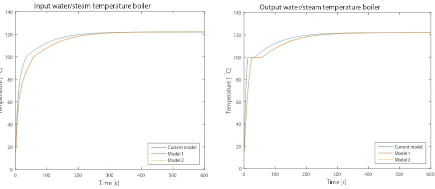
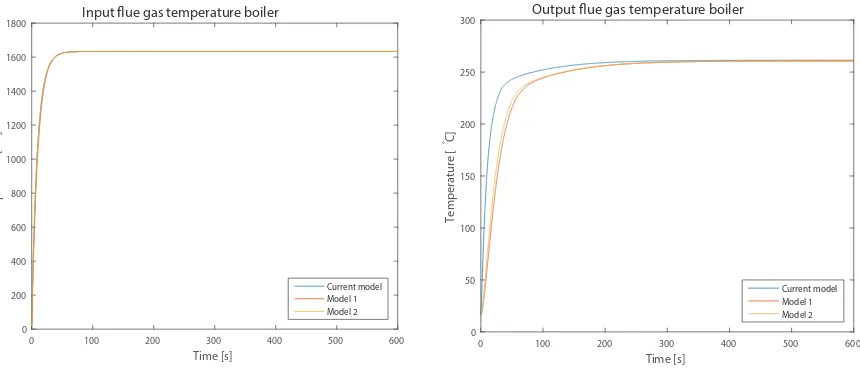
For the boiler the temperature plots are shown in figures 5.1 to 5.4. The mass flow of wa-ter/steam is 30 kg/s and the mass flow of the flue gas is set to 2.5 kg/s. The surface area for heat exchange is 360 m2. For model 1 and 2 a mass of 650 kg was used for the wall, with a specific heat for steal of 0.477 kJ/kgK. The number of elements used in this models is 20.

Time [s]

0 100 200 300 400 500 600

Temperature [

°C]

0 20 40 60 80 100 120 140

Input water/steam temperature boiler

[image:16.595.82.516.263.452.2]

Current model Model 1 Model 2

Figure 5.1: Input temperature water/steam

Time [s]

0 100 200 300 400 500 600

Temperature [

°C]

0 20 40 60 80 100 120

140 Output water/steam temperature boiler

Figure 5.2: Output temperature water/steam

(17)

Time [s]

0 100 200 300 400 500 600

Temperature [ °C] 0 200 400 600 800 1000 1200 1400 1600

1800 Input flue gas temperature boiler

[image:17.595.85.515.88.275.2]

Figure 5.3: Input temperature flue gas

Time [s]

0 100 200 300 400 500 600

Temperature [ °C] 0 50 100 150 200 250 300

Output flue gas temperature boiler

Figure 5.4: Output temperature flue gas

The output temperature of flue gas side shows the same phenomena as described above for the water/steam side.

Time [s]

0 100 200 300 400 500 600

Heat exchange [kJ/s]

-1000 0 1000 2000 3000 4000

5000 Heat exchange water/steam side boiler

[image:17.595.84.517.352.537.2]

Figure 5.5: Heat exchange water/steam side

Time [s]

0 100 200 300 400 500 600

0 500 1000 1500 2000 2500 3000 3500 4000 4500

5000 Heat exchange flue gas side boiler

Figure 5.6: Heat exchange flue gas side The heat exchange of both sides is quite similar for all the models. Models 1 and 2 are showing some delay on the water/steam side, because of the capacitance of the wall.

Comparing the outcomes of the three models, it can be noticed that the results are quite similar. The influence of the wall mass is visible in the results and no instabilities have been found.

(18)

Nodes

0 2 4 6 8 10 12 14 16 18 20

Temperature [

°C]

0 200 400 600 800 1000 1200 1400 1600

1800 Temperature per element boiler

Water/steam Flue gas Wall

Figure 5.7: Temperature model 1

Nodes

2 4 6 8 10 12 14 16 18 20

Temperature [

°C]

0 500 1000

1500 Temperature per element boiler

[image:18.595.84.516.85.263.2]

Figure 5.8: Temperature model 2 Both models are showing simular results.

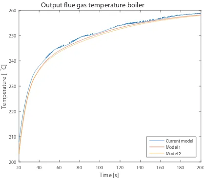
In case there is an instability introduced in the input of the water/steam side of the heat exchanger (figure 5.9), the output of the LMTD model will also suffer from this instability while the other models do not have this problem(figure 5.10).

Time [s]

20 40 60 80 100 120 140 160 180 200

Temperature [

°C]

80 85 90 95 100 105 110 115

120 Input water/steam temperature boiler

[image:18.595.79.287.367.551.2]

Time [s]

20 40 60 80 100 120 140 160 180 200

Temperature [

°C]

200 210 220 230 240 250 260

Output flue gas temperature boiler

[image:18.595.306.515.368.552.2]

(19)

5.2 Superheater

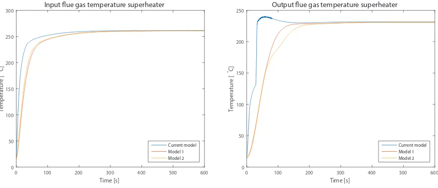
Figures 5.11 to 5.14 are showing the temperature of the superheater over time. The superheater has an area of 100m2 and a wall mass of 180kg. When the water in the drum becomes vapor a flow of steam enters the heat exchanger. The output stream of the flue gas from the boiler is the input for the superheater.

Time [s]

0 100 200 300 400 500 600

Temperature [ °C] 0 20 40 60 80 100 120 140

Input water/steam temperature superheater

Time [s]

0 100 200 300 400 500 600

Temperature [ °C] 0 50 100 150 200 250

300 Output water/steam temperature superheater

Figure 5.12: Output temperature wa-ter/steam

The figures show that the input and output temperatures of model 1 and 2 are delayed in comparison with the temperatures of the LMTD model. This could be explained by the heat capacitance of the wall and the fact that in model 1 and 2 the water is boiling slightly later. In contrast to the other models, model 1 shows no constant output temperature at boiling point. This can be explained by the procedure at low mass flows where the output temperature is approximated with the temperature of the wall.

Time [s]

0 100 200 300 400 500 600

Temperature [ °C] 0 50 100 150 200 250

300 Input flue gas temperature superheater

Time [s]

0 100 200 300 400 500 600

Temperature [ °C] 0 50 100 150 200

250 Output flue gas temperature superheater

[image:19.595.81.517.157.374.2]

[image:19.595.81.515.489.676.2]

(20)

Time [s]

0 100 200 300 400 500 600

0 20 40 60 80 100 120

140 Heat exchange water/steam side superheater

Time [s]

0 100 200 300 400 500 600

0 50 100 150 200 250 300

Heat exchange flue gas side superheater

[image:20.595.82.514.87.275.2]

Figure 5.16: Heat exchange flue gas side

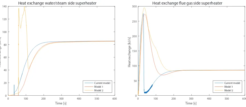
In figure 5.15 model 2 shows some large peaks of heat exchange for the water/steam side between 50 and 120 seconds. This is caused by a combination of low mass flows, a transition of water and steam and a heat transfer coefficient which is only dependent of mass flow. The mass of the fluid, which is chosen as a constant, and the use of values form the previous time step could cause some problems as well. But these peaks did not cause instabilities. The heat exchange at the flue gas side looks a bit different for the LMTD model than for the other models, as in the LMTD method the heat capacity of the wall is not included.

The temperature development over the nodes for model 1 and 2 at 600 seconds is shown in figures 5.17 and 5.18.

Nodes

0 2 4 6 8 10 12 14 16 18 20

Temperature [ ° C] 120 140 160 180 200 220 240 260 280

Temperature per element superheater

Nodes

2 4 6 8 10 12 14 16 18 20

Temperature [ °C] 120 140 160 180 200 220 240 260 280

Temperature per element superheater

[image:20.595.84.517.452.642.2]

(21)

Nodes

0 2 4 6 8 10 12 14 16 18 20

Temperature [

° C]

100 150 200

250 Temperature per element superheater

[image:21.595.89.514.87.267.2]

Nodes

2 4 6 8 10 12 14 16 18 20

Temperature [

°C]

80 100 120 140 160 180 200 220 240

260 Temperature per element superheater

[image:21.595.299.517.87.262.2]

The number of elements chosen in model 2 has little influence on the output temperatures of the heat exchanger, as shown in figures 5.21 and 5.22. In case the number of elements decrease, the volume of the discrete element will increase. This change in volume of the element has influence on the heat transfer within the element. The heat transfer coefficient of both fluids has been changed, in order to obtain the same temperatures at the end of a run (at 600 seconds). The mass of the fluids have been increased as well, to obtain a stable situation with less elements.

Time [s]

0 100 200 300 400 500 600

Temperature [

° C]

0 50 100 150 200 250

300Output temperature water/steam side superheater

5 elements 10 elements 20 elements

Time [s]

0 100 200 300 400 500 600

Temperature [

°C]

0 50 100 150 200 250

Output temperature flue gas side superheater

5 elements 10 elements 20 elements

[image:21.595.80.292.395.572.2] [image:21.595.296.516.395.571.2]

(22)

[image:22.595.169.432.166.388.2]

5.3 Economizer

Figures 5.23 to 5.25 show the temperature of the economizer over time. The economizer has an area of 400 m2 and a wall mass of 750kg. The level of the drum is regulated with a controller which changes the valve opening, in this way controlling the amount of water/steam flow through the economizer. The flow in front of the valve has a temperature of 104 °C and a pressure of 69.28 bar.

Time [s]

0 100 200 300 400 500 600

Temperature [

° C]

0 50 100

150 Output water/steam temperature economizer

Figure 5.23: Output temperature water/steam

A difference of output temperature between the LMTD model and the other models is shown in figure 5.23. The LMTD model did use the pressure of 69.28 bar in front of the valve, while the other models included the pressure drop over the valve.

Time [s]

0 100 200 300 400 500 600

Temperature [

° C]

0 50 100 150 200 250

Output flue gas temperature economizer

[image:22.595.81.520.494.675.2]

Time [s]

0 100 200 300 400 500 600

Temperature [

°C]

0 20 40 60 80 100 120

Output flue gas temperature economizer

(23)

Time [s]

0 100 200 300 400 500 600

-6000 -5000 -4000 -3000 -2000 -1000 0

1000 Heat exchange water/steam side economizer

[image:23.595.85.519.84.258.2]

Time [s]

0 100 200 300 400 500 600

-400 -300 -200 -100 0 100 200 300 400

Heat exchange flue gas side economizer

(24)

6 Reflection

6.1 Conclusion

The program PsxCad is continuously developing. During my internship a lot of changes have been made to improve the performance, stability and accuracy of the program. Regarding performance, model 1 is not useful as a model for the heat exchanger, the iterative calculations cost too much computational power. Model 2 is more suitable as an advanced heat exchanger model. Including the heat capacitance of the wall and the discretization of the heat exchanger in smaller elements lead to more stable and realistic results during the startup compared to the LMTD model. In the new model the number of initial values and process parameters is increased, the process parameters makes the setup of the process becomes more difficult. But on the other hand there a more possibilities to fine tune the process.

6.2 Recommendations

There are several shortcomings concerning the models. For example, in all the models we decided to consider the heat transfer coefficient being only dependent of the mass flow. In order to get a more realistic result this coefficient should be dependent of more fluid parameters, although this will lead to more complexity. In addition, only convection is taken into account in the model, conduction and radiation is neglected.

In model 2 the mass of the fluid is regarded as a constant, meaning that changes in the state of the fluid are not being taken into account. Considering the mass as a constant factor leads to more stability, but sometimes unrealistic results. The LMTD model and model 2 are using values from the previous time step, which could cause instabilities. Decreasing the time step could reduce the change of instabilities.

Another shortcoming of the heat exchanger models could be the fact that different elements have been put together in one block, making it difficult to change flow directions. By splitting all those elements into a network of separate blocks, it might be easier to make different configurations of a heat exchanger, like a co flow heat exchanger.

6.3 What I have learned

(25)

Appendices

A

Flue gas formulas

For the flue gas side of the heat exchanger specific enthalpy, specific heat capacity and temper-ature are parameters which are often used in the models. The enthalpy and heat capacity can be calculated using the NASA polynomials.

Hi

R·T =a1,i+ a2,i·T

2 +

a3,i·T2

3 +

a4,i·T3

4 +

a5,i·T4

5 +

a6,i

T (A.1)

Cp,i

R =a1,i+a2,i·T+a3,i·T

2₊_a

4,i·T3+a5,i·T4 (A.2)

Where a1, a2, a3,a4,a5 and a6 are the numerical coefficients for each component iof the flue

gas, T is the temperature in Kelvin andR is the universal gas constant.

By rewiring and including the molar mass of the component the specific enthalpy and specific heat capacity can be found.

hi =Mi·R·

h

a1,i·T +

a2,i

2 ·T

2₊a3,i

3 ·T

3₊a4,i

4 ·T

4₊a5,i

5 ·T

5₊_a 6,i

i

(A.3)

cp,i =Mi·R·

h

a1,i+a2,i·T +a3,i·T2+a4,i·T3+a5,i·T4

i

(A.4)

In order to reduce calculation time, the molar mass and the universal gas constant can be included into the constantsa1 - a6.

The specific enthalpy and specific heat capacity of the mixture can be calculated as follows, whereyi denotes the mass fraction of the component in the flue gas:

h=X

i

yi·hi (A.5)

cp =

X

i

yi·cp,i (A.6)

The function for calculating the specific heat as described above was already in use in PsxCad. For the specific enthalpy another function was used which was based on cp=dh/dT. However,

this function uses twice as much computational power, by using the enthalpy calculation twice, in comparison with the specific heat capacity calculation with the polynomials.

cp(T) =

h(T+ 0.3)−h(T−0.3)

0.6 (A.7)

There is not such a polynomial to calculate the temperature for the corresponding enthalpy h. An iterative method, based ondT =dh/cp, can be used to approximate the temperature. First

a reference temperature ofT0= 25°C is chosen and then h0 and cp,0 can be determined.

∆ho=h−ho (A.8)

T∗=T0+

∆h0

cp,0

(26)

With this new temperature a corresponding c∗_p can be determined with the cp function. And

an averagecp value can then be calculated.

¯

cp=

cp,0+c∗p

2 (A.10)

With this average specific heat coefficient a new temperature can be calculated.

T∗=T0+

∆h0

¯

cp

(A.11)

By using this calculated temperature a corresponding enthalpy can be found and a difference between this enthalpy value and the provided enthalpyh can be calculated.

∆h∗=h∗(T∗)−h (A.12)

A new temperature guess can be made.

T∗=T0+

∆h0−∆h∗

¯

cp

(A.13)

Finally, the new enthalpy difference become:

∆h∗= ∆h∗+h∗(T∗)−h (A.14)

The calculation for the temperature is the same as (A.13).

(27)

References

[1] Powerspex, 2016. http://www.pwerspex.nl/.

[2] Johan Schmaal, 2015. Powerpoint PSX Training simulator for Power stations.

[3] Joan Soler Fossas. Modelling of multistream lng heat exchangers. Master’s thesis, Norwe-gian University, June 2011.

[4] Stian Aaltvedt. Optimal operation of parallel heat exchanger networks. Master’s thesis, Norwegian University, June 2013.

[5] B. Beauchamp L. Lamarche and S. Kajl. A dynamic model of a vertical direct expansion ground heat exchanger.

[6] Wilfried Visser. Generic analysis methods for gas turbine engine preformance. Master’s thesis, University of Delft, 2014.

[7] Satyam Bendapudi. Dynamic modeling of shell-and-tube heat-exchangers: Moving bound-ary vs. finite volume, 2004.

[8] Iain Nicholas Grace. Modelling the preformance and dynamics of vapour compression refrigeration systems. Master’s thesis, Brunel University, January 2000.

[9] Amimul Ahsan. Evaporation, condensation and heat transfer. InTech, 2011.