3D printed implementation of a tactile force sensor working in multiple DOF

2.1 Schematic of whisker. A forceFext is applied at a distance sfrom the base of

the whisker. . . 3

2.2 Model of 2DOF-sensor. The beam is clamped at both sides and the whisker is connected at the centre. . . 4

2.3 Free body diagram of 2DOF-sensor with all moments and forces displayed. . 5

2.4 Top view of 4DOF sensor. The beams have been numbered for analysis and results purposes. The star indicates the position of the whisker. . . 6

2.5 Moments and the axes they belong to in a three dimensional system. . . 6

2.6 Exaggerated example of shear strain caused by external force Fext,y . . . 7

2.7 Exaggerated example of a twisted bar. One part of the beam will not rotate due to its constraint. The other end of the beam will rotate with this angleθx [7]. . . 8

2.8 Distribution of shear stress in rectangular beam [9]. . . 8

2.9 Free body diagram of the whisker . . . 10

2.10 The four different modes of deformation. . . 11

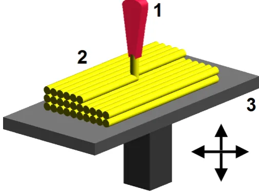
3.1 FDM printing process[16] . . . 15

3.2 Warping due to the cooling of the print [15] . . . 16

3.3 Design of the 2DOF sensor. . . 16

3.4 Design of the 4DOF sensor. . . 17

3.5 3D-printed 2DOF-sensor. . . 17

4.1 Measuring setup to measure the angle and the deflection. A force of 1 N is applied to the whisker. . . 18

4.2 Example of possible results from angle analysis. . . 19

4.3 Deflection 4DOF-sensor when a force Fext of 2 N is applied . . . 20

4.4 Deflection 4DOF-sensor when a force Fext of 2 N is applied . . . 20

4.5 The effect of soldering done poorly. . . 21

5.1 Modelled moment versus calculations. . . 23

5.2 Deflection of the left beam for both sensors when a force of 2 N is applied to the whisker. . . 24

5.3 Strain gauge impedance analysis. . . 25

5.4 Resistance and capacitance for both strain gauges when a force is applied to the whisker. . . 25

x-direction. . . 28

5.8 Calculations for the two moments and forces when a force is applied in the y-direction. . . 29

A.1 Free body diagram of 2DOF-sensor with all moments and forces displayed. . 32

B.1 2DOF 3D-printed sensor. . . 36

B.2 4DOF 3D-printed sensor. . . 37

B.3 Detailed description of sensor. . . 37

List of Tables

5.2 Angles due to applied force for the 2DOF and 4DOF-sensor. . . 22

5.3 Angles due to applied force for the 2DOF and 4DOF-sensor. . . 23

5.4 Gauge factor values . . . 26

5.5 Error per sample . . . 27

5.6 Resistance and capacitance values for the 4 strain gauges numbered as in Ap-pendix B . . . 28

1 Introduction 1

1.1 Previous research . . . 1

1.2 Goals . . . 2

2 Modelling 3 2.1 Design . . . 4

2.2 2DOF-analysis . . . 4

2.3 4DOF-analysis . . . 6

2.3.1 Additional Force . . . 7

2.3.2 Torsional strain . . . 7

2.3.3 Reduction . . . 9

2.4 Resistive measurement . . . 12

3 Design fabrication 14 3.1 Fusion deposition modelling . . . 14

3.2 Filaments . . . 16

3.3 Software . . . 16

4 Methods 18 4.1 Angle . . . 18

4.2 Deflection . . . 19

4.3 Strain . . . 20

5 Results 22 5.1 Angle . . . 22

5.2 Deflection . . . 24

5.3 Strain . . . 24

5.3.1 2DOF . . . 24

5.3.2 4DOF . . . 28

6 Discussion 30 7 Conclusion and suggestions 31 7.1 Conclusion . . . 31

7.2 Suggestions . . . 31

Introduction

Humans feel by means of a huge network of nerve endings and touch receptors in the skin. This system is called the somatosensory system [1]. They are able to measure certain forces by using two different kinds of receptors. When the skin is touching an object, rapidly adapting touch receptors react instantly to it. It can sense when the skin is touching the object and when it stops. However, it cannot sense continuous pressure of the object touching the skin. This continuous pressure is sensed by slowly adapting touch receptors.

Animals that have whiskers mostly use them to investigate their environments for two reasons [2]:

1. They have bad eyesight

2. They have long snouts, which partially blocks their view

Nerve cells in their skin help them determine when something touches the whisker and thereby feel their surroundings. A clear example of the use of whiskers on animals can be found in the rat family. When a rat is moving it feels with the whiskers on both sides of its head whether there is an object in its way. If an object is encountered, rats use their whiskers to explore the object [3]. The idea of having a whisker which is able to measure an object touching it gives rise to a lot of applications. An application that will be explored in this report is the use of whiskers as tactile force sensors.

In this report both a 2DOF and 4DOF-sensor will be modelled, tested and evaluated. The sensors will be 3D-printed. The number of people owning a 3D-printer keeps increasing which makes 3D-printed sensors more appealing. 3D-printing enables the user to print small and very accurate structures. Besides, faulty parts can easily be reprinted to increase the lifetime of the sensor. More about the (dis-)advantages of 3D-printing can be found in section 3.

1.1

Previous research

between certain surfaces, although there is still room for improvement. A whisker inspired sensor consisting of a flexible beam, torque sensor and actuator is considered in [5], where data show that straight-lined whiskers can be used to successfully distinguish surfaces while curved whiskers can not do so.

1.2

Goals

Modelling

To work towards the 4DOF-model, first the 2DOF-model is considered after which the effects of increasing the degrees of freedom are investigated. As Figure 2.1 implies, a force Fext is applied to the whisker at a distancesfrom the base of the whisker. When this force is applied two things will happen:

1. The base of the whisker will be displaced horizontally

2. The base of the whisker will rotate (a moment is created)

From the horizontal displacement the force acting on the whisker can be found, while the moment can be found from the rotation. When these two parameters are known the point of action can be determined.

2.1

Design

The beam that will displace horizontally due to the applied forceFext can be considered as a translational spring. By determining the stiffness of this spring the force can be found using Hooke’s law. The sensor will be stationary which means that it can be modelled as a beam clamped on both sides with the whisker connected in the center. Regarding the shape of the horizontal beam the most obvious choice would be to use a rectangular beam. The whisker can be connected perfectly onto the beam. This means that there will definitely be no extra effects due to e.g. the whisker not being fully connected.

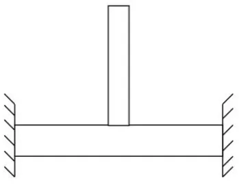
The moment can be measured from the rotational stiffness of the beam. Due to the applied force the beam will bend. The strain, which is created by this bending, can be measured by using two strain gauges. Those strain gauges are located at the top of the horizontal beam on each side of the whisker. A model of the deflection of the beam from which the force and moment can be determined has to be set up. Figure 2.2 shows the horizontal beam which is clamtped on both sides with the whisker connected in the center.

Figure 2.2: Model of 2DOF-sensor. The beam is clamped at both sides and the whisker is connected at the centre.

2.2

2DOF-analysis

Figure 2.3: Free body diagram of 2DOF-sensor with all moments and forces displayed.

The deflection of both parts of the beam due to an applied external force is given by:

w(x) = (_M0

EI

−1 8x

2₊ 1 4Lx

3 _{(x <} L

2) M0 EI n −5 8x

2₊ 1 4Lx

3₊xL

2 −

L2 8

o

(x > L₂) (2.1) which leads to the two strains given by:

εL=

M0 EI

2

54L4_s−45LL3_s + 10L2L2_s 960L2 +h 2 M0 EI −1 4 + 3 2LLs

+ Fext 2EA

εR=

M0 EI

2_54L4

s−45LL3s + 10L2L2s 960L2 −h 2 M0 EI −1 4 + 3 2LLs

− Fext

2EA (2.2)

2.3

4DOF-analysis

For the 4DOF-analysis the effects of increasing the DOF on the already existing 2DOF-analysis are considered. Before that, first, a new schematic will be constructed.

Figure 2.4: Top view of 4DOF sensor. The beams have been numbered for analysis and results purposes. The star indicates the position of the whisker.

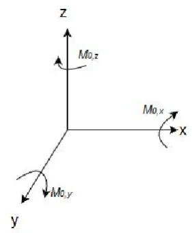
Besides, the moments have to be defined. As portrayed by Figure 2.5, the moments rotate around their corresponding axes.

Figure 2.5: Moments and the axes they belong to in a three dimensional system.

ε1 =

M0,y EI

2

54L4_s−45LL3_s + 10L2L2_s 960L2 +h 2 M0,y EI −1 4+ 3 2LLs

+Fext,x 2EA

ε3 =

M0,y EI

2

54L4_s−45LL3_s + 10L2L2_s 960L2 −h 2 M0,y EI −1 4+ 3 2LLs

−Fext,x

2EA (2.3)

2.3.1 Additional Force

The effects of having an forceFext,y on strain gauges 1 and 3 will be analysed. When a force is applied in the y-direction (e.g. from gauge 2 to gauge 4) strain gauges 1 and 3 will both move in the y-direction and have a certain rotationM0,x at the bottom of the whisker.

The displacement will give a certain shear strain. The shear stresses causing this shear strain do not aim to change the length of surfaces in all directions [6]. This means that the distance between the right side of beam 3 and the center of the whisker does not change.

Figure 2.6: Exaggerated example of shear strain caused by external forceFext,y

The angle, however, will change, resulting in a shear strain. The horizontal displacement, g in Figure 2.6, for strain gauges 1 and 3 is given as Fext,yL

4EA . The length in the x-direction is L

2 which gives the following angle:

tan(γshear)≈γshear=

Fext,yL 4EA

L

2 = Fext,y

2EA (2.4)

2.3.2 Torsional strain

Figure 2.7: Exaggerated example of a twisted bar. One part of the beam will not rotate due to its constraint. The other end of the beam will rotate with this angleθx[7].

To find the torsional strain as a result of this angle the maximum stress at the top surface is considered. The maximum stress, as distributed as in Figure 2.8, relates to the Torque as [6, 8, 9]

τmax= T db2

3 + 1.8b d

(2.5)

The strain and this shear stress are related via the shear modulus of elasticityG[6].

γtorsion = τmas

G

= T

Gdb2

3 + 1.8b d

(2.6)

The torque can be found from the angle of twist θ, the shear modulus of elasticity G, the torsion constantJ and the length of the beam L₂ [10].

T = 2GJ θ

L (2.7)

Combining Equations 2.6 and 2.7 yields the following equation

γtorsion = 2J θ Ldb2

3 + 1.8b d

(2.8)

EquationA.20 can be used to make the strain dependent on the moment. The torsion constant J is equal to βdb3 [10]. In this equation β is a constant depending on the ratio between d and b.

γtorsion= 2βbM0 16EI

3 + 1.8b d

(2.9)

The torsional strainγtorsion and shear strain γshear are added to the equations for the strain from Equation 2.3.

ε1 =

M0,y EI

2

54L4_s−45LL3_s + 10L2L2_s 960L2 +Fext,x EA +h 2 M0,y EI −1 4+ 3 2LLs

+ Fext,y 2EA +

2βbM0,x 16EI

3 + 1.8b d

ε2 =

M0,x EI

2

54L4_s−45LL3_s + 10L2L2_s 960L2

+Fext,x 2EA +h 2 M0,x EI −1 4+ 3 2LLs + Fext,y EA + 2βbM0,y 16EI

3 + 1.8b d ε3 = M0,y EI 2

54L4_s−45LL3_s + 10L2L2_s 960L2 −Fext,x EA −h 2 M0,y EI −1 4+ 3 2LLs

+ Fext,y 2EA +

2βbM0,x 16EI

3 + 1.8b d

ε4 =

M0,x EI

2

54L4_s−45LL3_s + 10L2L2_s 960L2

+Fext,x 2EA −h 2 M0,x EI −1 4+ 3 2LLs

− Fext,y

EA +

2βbM0,y 16EI

3 + 1.8b d

(2.10)

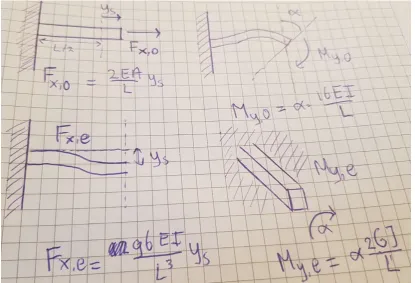
2.3.3 Reduction

However, section 2.3.1 is only true under one assumption which does not hold for this sensor. The horizontal deflection for the 2DOF-sensor was given as Fext,xL

4EA . For the 4DOF-sensor two

Figure 2.9: Free body diagram of the whisker

The free body diagram of Figure 2.9 is used to construct equations for the force and moment balance. The odd and even numbered forces and moment will be split. This decision was made because the odd terms experience the same behaviour and the even terms as well. The balances are given as:

X

Fx=F + X 0=1,3

Fo,x+ X

e=2,4 Fe,x

X

My =−F∗s+

X

i=1,2,3,4

My,i (2.11)

The force is delivered from strain gauge 1 to strain gauge 3 which means that the forces have opposite sign. The forces for strain gauges 2 and 4 do have the same sign:

Fx,1=−Fx,3=Fx,o Fx,2=−Fx,4=Fx,e

(2.12)

αi=α (2.13) Filling in the equations of 2.12 and 2.13 into the balance equations gives the following two equations:

Fx+ 2Fx,o+ 2Fx,e= 0

−Fxs+ 2My,o+ 2My,e= 0

(2.14)

Figure 2.10 shows the possibilities of deformation for each beam. In this case a force is applied from beam 1 to beam 3. Beams 1 and 3 will therefore elongate, following the upper left mode. The beams will bend asymmetrically around the whisker following the upper right mode. Beams 2 and 4 will follow the bottom two modes.

Figure 2.10: The four different modes of deformation.

Fx+4EA L ys+

192EI L3 ys= 0 Fx+ys

4EA L + 192EI L3 = 0

ys=− FxL

3

4EAL2_{+ 192EI} (2.15)

The same will be done for the moment balance, which will be written down in terms of the angleα.

−Fxs+ 32EI

L α+ 4GJ

L α= 0

−Fxs+ 32EI L + 4GJ L α= 0

α= FxsL

32EI+ 4GJ (2.16)

These values can be substituted back into the equations in figure 2.10 to obtain the reduction factors.

Fo,x= 2EA L ∗ −

FxL3

4EAL2_{+ 192EI} =−

EAL2

4EAL2_{+ 192EI}Fx Fe,x= 96EI

L3 ∗ −

FxL3

4EAL2_{+ 192EI} =−

24EI

EAL2_{+ 48EI}Fx My,o= 16EI

L ∗

FxsL 32EI+ 4GJ =

4EI

8EI+GJFxs

My,e= 2GJ

L ∗

FxsL 32EI+ 4GJ =

GJ

16EI+ 2GJFxs

(2.17)

To finish the model the parameters of Equation 2.10 should be replaced by their slightly reduced values.

2.4

Resistive measurement

The strain is measured by strain gauges located on top of the beams. By applying a force the beam, and therefore the strain gauge, either elongates or shortens creating a certain strain. This strain is related to the change in resistance by means of a gauge factor [11]. Each term of the strain equation will get their own gauge factor to improve the accuracy of the model.

∆R

R =GF ∗ε (2.18)

∆RL RL

=GFms1∗

M0 EI

2

54L4_s−45LL3_s + 10L2L2_s 960L2

+GFm1∗ h 2 M0 EI −1 4+ 3 2LLs

+GFf1∗ Fext 2EA

∆RR

RR =GFms2∗

M0 EI

2_54L4

s−45LL3s + 10L2L2s 960L2

−GFm2∗h

2 M0 EI −1 4+ 3 2LLs

−GFf2∗ Fext

2EA (2.19)

The three parameters can be found by using matrix inversion. The equations have to be rewritten in matrix form:

"_∆R L

RL ∆RR

RR # =     GFms1∗ 1 EI 2 54L4

s−45LL3s+10L2L2s 960L2

GFm1∗h₂M0

EI

−1₄ +₂3_LLs GFf1∗ _2EA1 GFms2∗

1

EI

2 54L4

s−45LL3s+10L2L2s 960L2

−GFm2∗ h₂M_EI0

−1 4 +

3

2LLs −GFf2∗

1 2EA      

M₀2 M0 Fext

 

(2.20) The three parameters can be found by taking the inverse of the 2x3-matrix. Since the matrix is not a square matrix there is no real inverse. A pseudo-inverse, which is a generalized version of the real inverse, will be taken. When M2

Design fabrication

The force sensor as modelled in the previous section will be 3D-printed. Before going into more detail about the design, shortly a contribution will be made regarding its (dis-)advantages and operation.

Before everyone can 3D-print i.e. sensors they have to purchase a 3D printer, unless they already own one. The Flashforge Creater Pro is used to print the upcoming designs. This printer prints using a method called Fusion Deposition Modelling, which will be abbreviated as FDM. Explanation regarding the operation of this method can be found in section 3.1. The costs of the filaments, which currently only come in plastic for this printing method, used in the printing are cheap compared to the price of the printer. Plastic can handle less stress compared to materials like steel, limiting the number of possibilities. For this project, however, plastic designs come in handy as they bend more easily.

Following, the 3D-printing process can take quite some time for not even very big structures. Especially when two different materials have to be printed sequentially with switching be-tween them. In section 3.1 more will be explained about this. According to P. Azimi et al. [13] particles released during printing might be toxic and exposure to these particles might cause health effects.

However, 3D-printing is not all that bad. Besides for the one time purchase of the printer, manufacturing of the product is cost wise attractive. Following, the user is free to choose what to print and can make his own designs very accurate [14].

3.1

Fusion deposition modelling

The printing process used in this BSc work is FDm. The Flashforge printer utilised in this research has 2 nozzles which means that in one print one is able to print a design with two different materials without replacing the filaments.

achieved the filament is pushed through the nozzle by the extruder. [15]

The two extrusion heads are connected to a system which is able to move the extrusion heads in the xy-plane, assuming the same coordinate system as in Figure 2.5. The melted material can because of this be deposited at a certain position. At this position the material cools down and solidifies, if necessary sped up with the use of fans connected to the extrusion head.

When the first layer has been printed and cooled down successfully, the printer bed will move down and the second layer will be printed on top of the already existing layer where they ”fuse”. If there has to be a switch between the materials, e.g. nozzle 1 has to cool down and nozzle 2 has to warm up. In the Gcode of the printer the nozzle will first cool down before the other nozzle can warm up. This is to prevent material to drip out of the first nozzle while printing with the second nozzle. The nozzle which prints the conductive TPU in this research has a diameter of 0.8 mm and the nozzle which prints the Ninjaflex has a diameter of 0.6 mm. More about the filaments can be found in section 3.2. In the design process this nozzle diameter should be considered. Sections with a width smaller than those diameters can not be printed.

Figure 3.1 shows the FDM printing process. The extruder, number 1, deposits the melted thermoplastic on the movable printer bed.

Figure 3.1: FDM printing process[16]

Figure 3.2: Warping due to the cooling of the print [15]

3.2

Filaments

Two different types of filaments are used, a conductor and an insulator. A conductive TPU, PI-ETPU 95-250 carbon black - 1.75 mm diameter , is used for the conductive parts (black) showed in Figures 3.3 and 3.4. This filament has a tensile modulus of 12 MPa [17]. The insulator parts of the design are printed with Ninjaflex 85A TPU. Its tensile modulus is also 12 MPa [18].

3.3

Software

The designs are made in the environment Autodesk Fusion 360 [19]. For the 2DOF sensor the following model has been created:

Figure 3.3: Design of the 2DOF sensor.

The downside of using prime pillars, as discovered during printing, is that prime pillars get loose from the printing bed easily and therefore get dragged along with the extrusion head. This can be solved by increasing the size of the prime pillar. However, this yields a very large increase in printing time.

The 4DOF-sensor is similar to the sensor. The half square enclosure from the 2DOF-sensor has been made a full square and now also beams are in the y-direction. The length of the strain gauge has been reduced slightly in order to prevent short circuiting with any other strain gauge. Four screw holes have been implemented in order to make the design more firm.

Figure 3.4: Design of the 4DOF sensor.

Figure 3.5 shows the 3D-printed 2DOF-sensor. In Appendix B both 3D-printed sensors can be found. Besides, a more detailed description can be found.

Methods

4.1

Angle

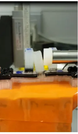
Both the electrical and mechanical model will be tested to validate the model for both the 2DOF and 4DOF-sensor. To test the mechanical model the angle and the deflection will be filmed. The Matlab function ”ginput” [20] will be used to analyse these films. This function puts a crosshair over the picture to be identified. The crosshair can be positioned at the desired position and by means of a mouse click the (x,y)-position is returned. The measuring setup of figure 4.1 is used to film the angle and deflection. The orange tape is used for two purposes:

1. Construct a firm setup such that the whisker of the sensor is on the proper height. This is done in order to ensure that the linear actuator actually exerts a force on the whisker.

2. Ensure that the entire sensor does not move when a force is applied to the whisker.

For the angle ginput(2) will be used which means two x,y-positions are returned. Figure 4.2 gives a demonstration of a possible result from this function, where positions 1 and 2 are returned by the function.

Figure 4.2: Example of possible results from angle analysis.

The angle can then be found using the inverse tangent:

Angle= arctan

ymax−ymin xmax−xmin

(4.1)

4.2

Deflection

A similar setup will be used to measure the deflection of the left beam. The deflection is antisymmetric around the bottom of the whisker, which is why both beams show the same deflection but with a different sign. The deflection of the left beam will be analysed. The deflection can be modelled using equation 2.1. In this model there is one unknown,M0. This moment can be modelled as the cross product between the forceFext and the point of action s[21].

M0=~s×Fext~

=||s|| · ||Fext||sinθ (4.2)

Figure 4.3: Deflection 4DOF-sensor when a force Fext of 2 N is applied

4.3

Strain

Figure 3.3 shows the 3D-printed 2DOF-sensor. From this design a circuit will be made up. It is assumed that the enclosure of the sensor will not move in anyway when a force is applied to the whisker.

Figure 4.4: Deflection 4DOF-sensor when a force Fext of 2 N is applied

capaci-tance. This capacitance is caused by the way the design is printed. Looking at figure 3.1 a lot of parallel wire capacitances can be found. The total capacitance will be in the range of pF.

The measuring equipment consists of two parts. To find the resistance of the strain gauges an LCR-meter will be used. Theoretically, there will only be a change in resistance when the strain gauge is elongated or shortened by a force. This force will be exerted by a linear actuator.

The resistance of the strain gauges will be measured with an HP 4284A LCR-meter [22] using 4-point measurements. As can be seen in Figures 3.3 and 3.4 each strain gauge has two ter-minals. Two wires will be connected to each terminal. On the left terminal the low current and low potential coming from the LCR-meter are connected, where the high potential and high current are connected to the right terminal. The shield of the four wires are connected to each other at the end. More information regarding the operation of the LCR-meter can be found in [22].

At one part of the wire a header pin is soldered and the other part is melted into the termi-nal. A slight disadvantage is that when one of these two processes is not done correctly it influences the results extremely. Figure 4.5 shows what happens when the soldering is done poorly. It seems that the soldering has an inductive effect on the impedance analysis. A force will be exerted on the whisker using the linear actuator SMAC LCA25-050-15F [23]. More information regarding the operation of SMAC actuators can be found in [24].

Results

For the analyses made in this chapter the following system parameters will be used:

Table 5.1: Parameter values

Parameter Value

E 12 MPa

A 9.6µm2

h 2 mm

Ls 22.5 mm

L 49.8 mm

b 2 mm

d 4.8 mm

β 0.249

5.1

Angle

Table 5.2 provides the results of the analysis for the angle of both sensors.

Table 5.2: Angles due to applied force for the 2DOF and 4DOF-sensor.

Force [N] θBottom,2DOF [◦] θBottom,4DOF [◦]

0 3.4778 2.5088

0.5 6.3402 5.7106

1 2.1390 10.6309

1.5 17.5779 14.8757

2 22.0151 18.7360

θ2DOF= 0.1686∗F orce+ 0.0462

Table 5.3: Angles due to applied force for the 2DOF and 4DOF-sensor.

Force [N] M0y,2DOF [N m] M0y,4DOF [N m]

0 0 0

0.5 0.0060 0.0060

1 0.0117 0.0118

1.5 0.0172 0.0174

2 0.0223 0.0227

M0y,2DOF= 0.0111∗θ2DOF+ 0.0003 M0y,4DOF= 0.0114∗θ4DOF+ 0.0002

(5.2)

In this equation the anglesθ2DOFandθ4DOF are given in radians. In the analysis of the 2DOF sensor the angle at the whisker was derived as a function of the momentM0. This was given as:

M0 = 16θEI

L (5.3)

5.2

Deflection

The mechanical model for the deflection will be tested in a similar fashion. A force of 2 N is applied to the whisker and the deflection is filmed. Besides, the model of equation 2.1 is used to compare the photographic results. In this model the value from Table 5.3 is used forM0y. The graph is obtained by using the ginput function with 16 samples.

(a) Model and photographic results of the de-flection for 2DOF-sensor with 16 samples.

(b) Model and photographic results of the de-flection for 4DOF-sensor with 16 samples.

Figure 5.2: Deflection of the left beam for both sensors when a force of 2 N is applied to the whisker.

5.3

Strain

5.3.1 2DOF

The resistance RL is equal to 71.250 kΩ and with a cutoff frequency of around 20 kHz this yields a capacitance of around 111.7 pF. The strain gauges are the same so the same resis-tances are expected. The resistance RR is equal to 79.536 kΩ and with a cutoff frequency of around 20 kHz this yields a capacitance of 100.5 pF.

(a) Impedance analysis for the left strain gauge.

(b) Impedance analysis for the right strain gauge.

Figure 5.3: Strain gauge impedance analysis.

(a) Resistance and capacitance when a force is applied to the whisker for the left strain gauge.

(b) Resistance and capacitance when a force is applied to the whisker for the right strain gauge.

Figure 5.4: Resistance and capacitance for both strain gauges when a force is applied to the whisker.

(a) Change in resistance and capacitance due to an applied force for the left strain gauge.

(b) Change in resistance and capacitance due to an applied force for the right strain gauge.

Figure 5.5: Resistance and capacitance change for both strain gauges when a force is applied to the whisker.

Comparing the different subplots of Figure 5.5 it can clearly be seen that the resistance in-creases step-wise as well. Less clear from the picture is that also the capacitance changes step-wise. For both it can be seen that the change becomes bigger when the force is bigger as well. From the strains the moment and force can be calculated. From this the point of action can be calculated. These results are displayed in Figure 5.6.

The parameters of Table 5.4 were used to obtain the results in Figure 5.6. The first two subplots both shows the moment M0. The first one is calculated by taking the square root of M₀2, while the second one is a direct calculation ofM0.

Table 5.4: Gauge factor values

Parameter Value GFms1 2 GFms2 15

GFm1 0.002

GFm2 0.001

Figure 5.6: Moment, force and point of action model and calculations.

Table 5.5 provides the error per sample for both the moment and the force. This average error per sample is obtained by dividing the total error by the number of samples.

Table 5.5: Error per sample

Parameter Average error

M0 0.0023 N m

5.3.2 4DOF

The strain gauges with dimensions as in Appendix B have valuesR and C as given in Table 5.6. The cutoff frequency for the strain gauges range from 11.5 kHz to 20.0 kHz.

Table 5.6: Resistance and capacitance values for the 4 strain gauges numbered as in Appendix B

Strain gauge Resistance [kΩ] Capacitance [nF]

1 5.33 1.49

2 19.7 0.70

3 37.1 0.24

4 33.7 0.26

For the 4DOF measurements a force will applied up to 2N (again the staircase with steps of 0.5 N).

Figure 5.8: Calculations for the two moments and forces when a force is applied in the y-direction.

Table 5.7: Values for the gauge factors of the 4DOF sensor strain equations

Strain gauge GFmsy GFmy GFmsx GFmx GFfy GFfx

1 1 1 * 1 100 0.01

2 * 1 1 1 100 1

3 1 1 * 1 1 1

4 * 1 1 1 100 1

Discussion

According to the theory, the angle should be smaller for the 4DOF-sensor due to the reduction of the parameters. Table 5.2 shows that the angle in fact is smaller for the 4DOF-sensor. The angles for the two sensors are used to construct relations between the moment and angle of the whisker. For the 2DOF-sensor this is compared to the model, Equation A.20. Figure 5.1 shows that the experimental data is much smaller than the model.

Subsequently, it can be seen that the deflection is also lower for the 4DOF-sensor. However, the deflection of the 4DOF-sensor follows the 2DOF-model better than the 2DOF-sensor which partially disproves the previous claim.

The strain analysis shows that the 2DOF-sensor does follow the proposed model. There seems to be a reasonably big error betweent= 5 s andt= 10 s, which can clearly be seen in the last subplot. The point of action shows values which are nearly four times as high as modelled. The 2DOF-sensor does seem to follow the model better aftert= 10 s.

The 4DOF-sensor, however, does not follow the model at all. It does not really matter in which direction the force is applied. Both figures 5.7 and 5.8 show that there is no similarity between the model and the experiment.

Conclusion and suggestions

7.1

Conclusion

The main goal was to see how 3D-printing could be used to make whisker inspired tactile sensors. Two similar sensors have been designed to investigate this. The 2DOF-sensor, as designed in this research, works with a certain margin of error. The average error in force is 0.1968 N on a stair case input with steps of 0, 0.5 and 1 N.

Although the 2DOF-sensor seems to work really well this cannot be said for the 4DOF-sensor. The data retrieved by the 4DOF-sensor seems to be more random. The goal to figure out how 3D-printing can be used to make whisker inspired tactile sensor thus failed partially.

7.2

Suggestions

The main thing to think about is how to get the 4DOF-sensor working properly. In the dis-cussion section multiple ideas were provided about things that could be wrong (model, gauge factors, measurements, 3D-print). To check whether the model is wrong each individual as-pect should be tested individually. However, this solution might be tricky as most parameters influence all beams.

A time-consuming solution for the gauge factor might be to check all possibilities in a certain range and check the total error. With 20 different gauge factors this might take a while or only a small range can be investigated.

Deflection derivation 2DOF-sensor

Figure A.1: Free body diagram of 2DOF-sensor with all moments and forces displayed.

Due to the constraints on both sides there cannot be any vertical displacements at the ends, which means that there should be a balance between the vertical forces:

FL+FR = 0 (A.1)

If the moment balance is considered for i.e. the left boundary, so aroundx= 0, the following equation is found:

ML−M0−MR+FR∗L (A.2)

To find both the internal shear force and the bending moment the beam is cut in two parts. For the left part, for (x < a), the moment balance aroundx= 0 is given as:

FL−V(x) = 0

For the other part of the beam, for (x > a), the moment balance aroundx= 0 is given as:

FL−V(x) = 0

ML−M0−V(x)∗x−M(x) = 0 (A.4)

The vertical deflection of a beam can be found from the bending moment using [25]

EId 2_w(x)

dx2 =M(x) (A.5)

This yields the following two beam equations:

EId 2_w(x)

dx2 = (

ML−FL∗x (x < a)

ML−M0−FL∗x (x > a) (A.6)

The deflection can be found by integrating equation A.6 twice and dividing byEI

w(x) (

= _EI1 ₁ 2MLx

2₋1 6FLx

3_+C

1x+C2 (x < a) = _EI1 1₂(ML−M0)x2−1₆FLx3+C3x+C4 (x > a)

To find the integration constants the boundary conditions are considered. Assuming that the clamps show no deflection the following set of boundary conditions can be found:

w1(0) = 0 dw1(0)

dx = 0 w2(L) = 0 dw2(L)

dx = 0 (A.7)

Besides, at position x = a there should be a continuous transition between the two parts of the beam, yielding the following two boundary conditions.

w1(a) =w2(a) dw1(a)

dx =

dw2(a)

dx (A.8)

Choosing a to be equal to half the length of the beam the following equations are found for the deflection. w(x) = (_M 0 EI

−1₈x2₊ 1

4Lx3 (x < L

2)

M0

EI

n

To find the length of the beam in deflection the curve length is calculated using [26]: https: //en.wikipedia.org/wiki/Arclength

S= Z Ls

0 r

1 + dw(x) dx

2

dx (A.10)

It is assumed that the length of the top surface is equal to the length of the neutral axis. For small displacements this can be approximated as:

S ≈

Z Ls 0

1 +1 2 dw(x) dx 2 dx = M0 EI 2

54L5_s −45LL4_s+ 10L2L3_s 960L2

+Ls (A.11)

The strain therefore equals:

εL=

S−Ls Ls =

M0 EI

2_54L4

s −45LL3s + 10L2L2s 960L2

(A.12)

For the right side of the beam the deflection is the same so the same strain is found. Besides there is an extra addition of strain due to the fact that the strain gauge is located at the top of the beam. The strain at a distance z from the neutral axis is given by [6]:

ε=zd 2_w(x)

dx (A.13)

For the left side of the beam this gives a strain of

εL(x) =z M0 EI − 1 4 + 3 2Lx (A.14)

The average strain measured with a strain gauge of lengthLs is given by:

εmeasured,L= 1 Ls

Z Ls 0

εL(x)dx

= h 2 M0 EI − 1 4+ 3 4LLs (A.15)

The strain for the right side of the beam is the same but with opposite sign.

u(x) = (_F

extx

2EA (x < L

2)

Fext(L−x)

2EA (x > L

2) The displacement at the center of the whisker is thus:

u

L 2

=k∗Fext

= 4EA

L u (A.16)

The added strain due to this spring deflection is again given as the change in length compared to the original length:

εSpring=

FextL

4EA L

2

= Fext

2EA (A.17)

The left part will compress positively with the factor above while the right part will be in tension with this factor, giving rise to the following two total strains:

εL=

M0,y EI

2

54L4_s −45LL3_s+ 10L2L2_s 960L2 +h 2 M0 EI −1 4 + 3 2LLs + Fext 2EA

εR=

M0,y EI

2

54L4_s −45LL3_s+ 10L2L2_s 960L2 −h 2 M0 EI −1 4 + 3 2LLs

− Fext

2EA (A.18)

The rotation of the beam at the whisker, which is required for the 4DOF-analysis, is given as [25]:

tan(θ) = dw

dx (A.19)

For small anglestan(θ)≈θ which means the rotation around the whisker equals:

θ≈ dw(

3D-printed sensors

Below the 3D-prints for both the 2DOF and 4DOF sensors are depicted. Figure B.3 shows a detailed description of the model with a front-, side- and top-view of the beams on the sensor.

Figure B.2: 4DOF 3D-printed sensor.

[1] Skin Sense of Touch — Science Project, Science Lesson.https://learning-center. homesciencetools.com/article/skin-touch/. Accessed on 2018-06-23. Oct. 2017.

[2] Why Do Animals Have Whiskers? http://mentalfloss.com/article/83046/why-do-animals-have-whiskers. Accessed on 2018-06-23. Apr. 2018.

[3] How do whiskers work? http : / / www . discoverwildlife . com / british - wildlife / how-do-whiskers-work. Accessed on 2018-06-23.

[4] Max Lungarella et al. An Artificial Whisker Sensor for Robotics. Tech. rep. Accessed on 2018-06-23. Research Group of Complex Systems Engineering, Graduate School of Engineering Hokkaido University, Sapporo 060-8628, Japan, 2002.

[5] Makoto Kaneko and Toshio Tsuji. A Whisker Tracing Sensor for Manufacturing Ap-plication. Tech. rep. Accessed on 2018-06-23. Industrial and Systems Engineering, Hi-roshima University, Kagamiyama, Higashi-HiHi-roshima 739-8527, JAPAN, 2000.

[6] J. M. Gere. Mechanics of materials. 6th ed. Thomson, 2007.

[7] Torsion (mechanics). https : / / en . wikipedia . org / wiki / Torsion _ (mechanics). Accessed on 2018-06-29. June 2018.

[8] Strength of Materials- Torsion of Non Circular Section. https://www.scribd.com/ document/61684112/Strength-of-Materials-Torsion-of-Non-Circular-Section-Hani-Aziz-Ameen. Accessed on 2018-06-17.

[9] E. J. HEARN. TORSION OF NON-CIRCULAR AND THIN-WALLED SECTIONS. 3rd ed. Accessed on 2018-05-26. Butterworth-Heinemann, 1997.

[10] Torsion constant.https://en.wikipedia.org/wiki/Torsion_constant. Accessed on 2018-05-24. Feb. 2018.

[11] Measuring Strain with Strain Gages. http://www.ni.com/white- paper/3642/en/. Accessed on 2018-06-23.

[12] pinv Moore-Penrose pseudoinverse. https://nl.mathworks.com/help/matlab/ref/ pinv.html. Accessed on 2018-06-29.

[13] P. Azimi et al. “Emissions of Ultrafine Particles and Volatile Organic Compounds from Commercially Available Desktop Three-Dimensional Printers with Multiple Filaments”. In:Environmental Science & Technology, 50(3), pp.1260-1268. (2016).

[14] A. Pearson and J. Flynt. 10 Advantages of 3D Printing. http://3dinsider.com/3d-printing-advantages/. Accessed on 2018-06-20. 2018.

[16] Fused filament fabrication. https : / / en . wikipedia . org / wiki / Fused _ filament _ fabrication. Accessed on 2018-07-01.

[17] Palmiga - PI-ETPU 95-250 Carbon Black - 1.75 mm. https://www.creativetools. se / hardware / 3d - printers - and - accessories / filaments / flexible - filaments / pi-etpu-95-250-carbon-black. Accessed on 2018-06-21.

[18] Anon. NinjaFlex R 3D Printing Filament. https : / / ninjatek . com / wp - content / uploads/2016/05/NinjaFlex-TDS.pdf. Accessed on 2018-06-21. 2018.

[19] Cloud Powered 3D CAD/CAM Software for Product Design — Fusion 360.Autodesk. com. Accessed on 2018-06-20.

[20] gtext. https : / / nl . mathworks . com / help / matlab / ref / ginput . html. Accessed on 2018-06-25.

[21] Why is moment of a force calculated by cross product?https://physics.stackexchange. com / questions / 357255 / why is moment of a force calculated by cross -product. Accessed on 2018-06-30.

[22] Hewlett Packard. HP 4284A PRECISION LCR METER OPERA TION MANUAL. 6th ed. Accessed on 2018-06-21. 2018.

[23] LCA Series. http : / / www . smac - mca . com / lca - series - p - 15 . html. Accessed on 2018-06-21.

[24] SMAC Moving Coil Actuators. Accessed on 2018-06-21.

[25] Mechanics of Materials chapter 6 Deflection of Beams. http://web.ncyu.edu.tw/

~lanjc/lesson/C3/class/Chap06-A.pdf. Accessed on 2018-05-17.

[26] Arc length.https://en.wikipedia.org/wiki/Arc_length. Accessed on 2018-06-23.