Inter-Symbol Interference Prevention
techniques for Noise-based Frequency
Offset Transmit-reference Systems
T.H.F. Hartman
B.Sc. Thesis
June 2016
Supervisors:
M.SC. I. Bilal Dr. ir. A. Meijerink
Telecommunication Engineering Group Faculty of Electrical Engineering, Mathematics and Computer Science University of Twente
Summary
The Telecommunication group, at the University of Twente, is working under the WALNUT project, on developing new ways of communication using noise-based transmit-reference (TR) modulation. TR modulation is a technique where a linear combination of the spreading signal and the spread signal, separated by a small frequency offset, are sent over a channel. By using this technique, no complex receiver scheme has to be implemented, because the spreading signal is also received.
Contents
1. Introduction ... 4
2. Theory ... 5
2.1 AWGN ... 5
2.2 Inter Symbol Interference (ISI) ... 7
2.3 Different ISI prevention techniques ... 8
2.4 AWGN 2-Path ... 10
2.5 AWGN 2-Path Root Raised Cosine Pulse Shaping ... 11
2.6 AWGN 2-Path Guard Interval ... 12
2.7 AWGN Multipath ... 14
2.8 AWGN Multipath Root Raised Cosine ... 15
2.9 AWGN Multipath Guard Interval ... 15
3. Experimental procedure and results ... 16
3.1 AWGN ... 16
3.2 Reliability of BER ... 17
3.3 AWGN 2-path ... 17
3.4 AWGN 2-path Root Raised Cosine Pulse Shaping ... 19
3.5 AWGN 2-Path Guard Interval ... 20
3.6 Comparison of the different techniques on the 2-path ... 21
3.7 AWGN Multipath ... 23
3.8 AWGN Multipath Root Raised Cosine ... 25
3.9 AWGN Multipath Guard Interval ... 26
3.10 Comparison of the different techniques on the multipath ... 28
4. Evaluations ... 29
4.1 Conclusion ... 29
4.2 Recommendation ... 29
1. Introduction
The TE group is working, under the WALNUT project, on developing new techniques for establishing robust radio links in wireless sensor networks (WSNs) that operate in an extremely crowded radio spectrum, at very low power, using noise-based transmit-reference (TR) modulation [1][2]. TR is a low-powered spread-spectrum (SS) technique that sends a linear combination of the spreading signal and the spread signal, separated by a small frequency offset, so that at the receiver, no carrier regeneration is needed. Hereafter, the signal will be despread, by the receiver, by correlating the received signal with the same frequency-shifted version of itself. No complex receiver scheme has to be implemented, and therefore the reduced synchronization time that comes with this scheme, makes it a promising communication scheme in short-range transmissions for low data-rate applications sending only burst of traffic.
The wideband nature of the resulting radio signals make the technique robust to fading due to multipath propagation (MP). However, in propagations channels with large delay spreads, the performance of such a noise-based frequency-offset modulation (N-FOM) communication system will be reduced by inter-symbol interference (ISI). ISI in the system is caused by the MP, implying that the signals reach the receiving antenna by two or more paths with different time lags. The signals that arrive at different time instances are summed, which causes neighbouring symbols to interfere with each other. A standard representation of such a channel is a tapped delay line (TDL) [2]. The noise that arises in this channel is described as additive white Gaussian noise (AWGN). In 2015 a performance analysis of the N-FOM system in dense frequency-selective fading channels was carried out by Bilal [2]. In his paper, the effect of ISI was ignored due to an assumption which is only validfor particular environments. The results of his paper indicate that at a much larger delay spread, ISI can no longer be ignored. This was seen by the results of the simulation that show a drastic drop in the average bit error rate (BER) compared to the theoretical BER considering large delay spreads. These findings result in the need for this study to take a look at the impact of ISI prevention techniques, such as a guard interval and pulse-shaping by the use of a raised cosine or root raised cosine (RRC), on the performance of the system, by means of simulation. Several more techniques such as changing the modulation technique, maximum-likelihood sequence estimation and equalizers, can be found, however those techniques are beyond the scope of this report. The techniques mentioned before are chosen since they seemed most feasible after a small study that was done on the several techniques. The other techniques also meant a change in the modulation technique or a more complex receiver architecture, this was avoided because the technique should be easily implementable within the given time constraint.
2. Theory
2.1 AWGN
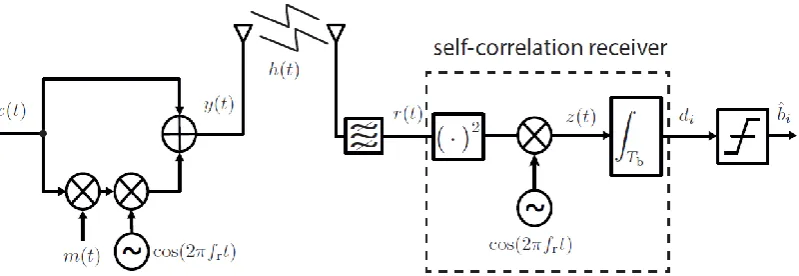
The N-FOM communication system in a multipath channel ℎ(𝑡), which was mentioned before, can be seen in figure 1 [2]. At the transmitter side, the spread signal 𝑥(𝑡) is multiplied with the message signal 𝑚(𝑡) and a frequency offset and to this multiplication 𝑥(𝑡) is also added, giving [3]
𝑦(𝑡) = 𝑥(𝑡) ∗ 𝑚(𝑡) ∗ cos(𝜔𝑟𝑡) + 𝑥(𝑡) (1)
The spreading signal 𝑥(𝑡) is modelled as a wide-sense-stationary Gaussian bandpass process centred around a RF frequency 𝑓𝑐. The transmitted signal 𝑦(𝑡) is then sent over the multipath
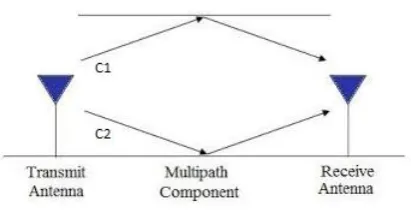
[image:5.595.101.501.407.545.2]channel ℎ(𝑡) which is represented by a TDL. At the receiver side, a front-end filter processes the received filter which is assumed to be a brick-wall filter such that it perfectly collects the TR signal and suppresses all out-of-band signals. The signal is then correlated with itself and multiplied with the same frequency offset that is used by the transmitter. The signal is then put through an integrate and dump filter (IDF) which functions as a matched filter for non-return-to-zero (NRZ) binary phase-shift keying (BPSK) square pulses. These NRZ BPSK square pulses are referred to in this paper as the general case, where no change has happened yet. To give a better understanding of the problems that are faced, figure 1 and these different steps will be called upon.
Figure 1: N-FOM communication system in a multipath channel ℎ(𝑡).
Bit Energy Calculation
The bit energy of the transmitted signal 𝑦(𝑡) is calculated to get a description of the theoretical value of the mean power of the spread signal, since the bit energy is a pre-defined value. For the calculation the following transmitted signal is used;
𝑦(𝑡) = 𝑥(𝑡) ∗ 𝑚(𝑡) ∗ cos(𝜔𝑟𝑡) + 𝑥(𝑡) ∗ 𝑐 (2)
𝐸𝑏 = 𝐸 [ ∫ 𝑦2(𝑡)𝑑𝑡 𝑘+𝑇𝑏
𝑘
]
= ∫ 𝑥2(𝑡)𝑚2(𝑡) cos2(𝜔
𝑟𝑡) + 2𝑥2(𝑡)𝑚(𝑡) cos(𝜔𝑟𝑡) + 𝑥2(𝑡) 𝑑𝑡 𝑘+𝑇𝑏
𝑘
= 𝑃𝑥 ∫
1 2𝑚
2(𝑡) +1
2𝑚
2(𝑡) cos(2𝜔
𝑟𝑡) + 2𝑚(𝑡) cos(𝜔𝑟𝑡) + 1 𝑑𝑡 𝑘+𝑇𝑏
𝑘
=1
2𝑃𝑥 ∫ 𝑝
2(𝑡)𝑑𝑡 𝑘+𝑇𝑏
𝑘
+ 𝑃𝑥 ∫ +
1 2𝑝
2(𝑡) cos(2𝜔
𝑟𝑡) + 2𝑝(𝑡) 𝑏0cos(𝜔𝑟𝑡) 𝑑𝑡 𝑘+𝑇𝑏
𝑘
+ 𝑃𝑥𝑇𝑏
Where the second integral turns to zero if 𝜔𝑟 is a multiple of 2𝜋
𝑇𝑏 giving,
=1
2𝑃𝑥𝑇𝑏+ 𝑃𝑥𝑇𝑏 𝐸𝑏 = 𝑃𝑥(
1
2𝑇𝑏+ 𝑇𝑏)
And since,
𝑃𝑦=
𝐸𝑏
𝑇𝑏
= 𝑃𝑥(
1 2+ 1)
Giving,
𝑃𝑥=
𝑃𝑦
(12 + 1)
For an optimal output of the system the energy of the information part and the energy of the spread signal part should be the same. Looking at this case it is seen that the spread signal part has twice than the energy of the information part. This can be compensated by dividing the spread signal part with the √2. Doing the same calculations with 𝑐 = 1
√2 gives:
2.2 Inter Symbol Interference (ISI)
Before going into the several techniques to actually prevent ISI, we first study ISI. ISI is the unavoidable consequence in our wireless communication where the same signal arrives with different time lags at the receiver. This effect is shown in the following figure [4].
Figure 2: (a) Transmitted signal, (b) Received signal.
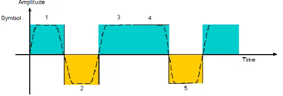
[image:7.595.103.331.146.302.2]In figure 2 (a) you can see that the symbols are transmitted as square waves separated by a relatively big time gap. At the receiver side however, figure 2 (b), the symbols are received all smeared. This smearing arises because several signals arrive at different times with reduced powers. In this figure the symbols are send with big delays between each other so that they don’t interfere. In a communication system the symbols are transmitted closer together as shown in figure 3. The fact that a gap between the different symbols reduces ISI already shows one promising technique, which is the guard interval technique. This technique implies that at the end of each bits some zeros are send. This drops the data rate but helps against the ISI.
Figure 3: Sequence 101101 to be transmitted.
[image:7.595.100.376.443.537.2]Figure 4: Sequence 10110 perceived at the receiver after spreading over time.
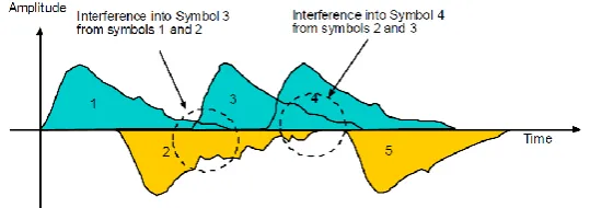
[image:8.595.95.365.79.174.2]In the figure it can be seen that where symbols change their polarity, interference into the symbols take place. 2 symbols with the same orientation interfere with each other but not in a detrimental way. The different symbols are now added and compared with the transmitted signal in the following figure.
Figure 5: Received signal vs. Transmitted signal.
The green line indicates the actually received signal, which represents all the different symbols from figure 5 added up. The dotted line represents the transmitted signal. It can be clearly seen that some of the symbols are influenced by their neighbouring symbols. Symbol 2 which is in between 2 symbols of different polarity is harmed a lot more than symbol 4, which is not preceded by a symbol of different polarity.
2.3 Different ISI prevention techniques
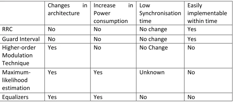
To actually prevent the detrimental effect of ISI, several ISI prevention techniques were studied. Here these techniques will be discussed and the reasons for choosing certain techniques will be given. As mentioned in the introduction the system should be able to operate in an extremely crowded radio spectrum, at very low power, with a low synchronization time. Using certain techniques could change some of the aspects of the system and therefore not keep these restriction. The time constraint, of this module, should also be taken into account and because of this, techniques with small changes are more preferable.
RRC
Guard Interval
For the Guard Interval technique only the message signal is changed by turning parts of the bits into zeros. For the architecture of the scheme no change is needed.
Higher-order Modulation Technique
The principle behind higher-order modulation is increasing the amount of information per symbol [5]. When doing so, the bit-rate is increased because more information is send in the same amount of time. If one would however keep the same bit-rate this would mean longer symbol times, which at its turn reduces ISI. Together with this technique, would also come some minor changes in the architecture.
Maximum-likelihood estimation
To implement maximum-likelihood estimation one would have to emulate the distorted channel. This would mean more power consumption and one would have to know which channel is involved which is a big con.
Equalizers
Equalizers are RX structures that work both ways: they reduce or eliminate ISI, and at the same time exploit the delay diversity inherent in the channel [6]. For an interpretation in the frequency domain, delay dispersion corresponds to frequency selectivity. In other words, ISI arises from the fact that the transfer function is not constant over the considered system bandwidth. The goal of an equalizer is to reverse distortion by the channel. The product of the transfer functions of channel and equalizer should be constant. Implementing equalizers would mean however, first of all, a big change in the architecture of the system and a lot of time to fully understand and implement them.
Changes in architecture
Increase in Power consumption Low Synchronisation time Easily implementable within time
RRC No No No change Yes
Guard Interval No No No change Yes
Higher-order Modulation Technique
Yes No No Change No
Maximum-likelihood estimation
Yes Yes Unknown No
[image:9.595.92.493.435.610.2]Equalizers Yes Yes No No
Table 1: Pros and cons of the ISI prevention techniques.
2.4 AWGN 2-Path
The general idea of the AWGN 2-path is to get a better understanding of the resulting ISI that arises because the 2 signals arriving at different time instances. The influence of this ISI on the BER is checked and will be discussed in the experimental procedure and results. The general idea of a two-path is represented in figure 6.
Meaning the different signals arrive at different times and where the channel is represented as
ℎ(𝑡) = 𝑐1𝛿(𝑡 − ∆𝜏1) + 𝑐2𝛿(𝑡 − ∆𝜏2) (3)
An important aspect of this 2-path is the fact that the mean power of the 2 transmitted signals should be equal or close to the mean power of the case were only one signal was send. At the receiver these 2 signals are received as a sum of the individual signals. The following calculations can be done that come with a restriction:
𝑦(𝑡) → 𝑃𝑦= 𝐸[𝑦2(𝑡)]
𝑦2−𝑝𝑎𝑡ℎ(𝑡) = 𝑐1𝑦(𝑡) + 𝑐2𝑦(𝑡 − 𝑇𝑑)
𝑃𝑦2−𝑝𝑎𝑡ℎ = 𝐸[𝑦2−𝑝𝑎𝑡ℎ2 (𝑡)]
𝑃𝑦2−𝑝𝑎𝑡ℎ = (𝑐1
2+ 𝑐
22)𝑃𝑦+ 2𝑐1𝑐2𝐸[𝑦(𝑡)𝑦(𝑡 − 𝑇𝑑)]
𝑃𝑦2−𝑝𝑎𝑡ℎ = (𝑐1
2+ 𝑐
22)𝑃𝑦+ 2𝑐1𝑐2𝑅𝑦(𝑇𝑑)
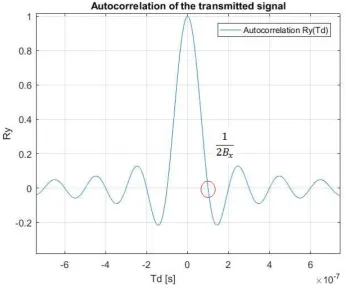
Where the autocorrelation 𝑅𝑦(𝑇𝑑) goes to 0 if 𝑇𝑑 ≥ 1
2𝐵𝑥 resulting in the following,
𝑃𝑦2−𝑝𝑎𝑡ℎ = (𝑐1
2+ 𝑐 22)𝑃𝑦
Since 𝑃𝑦should be considered equal to 𝑃𝑦2−𝑝𝑎𝑡ℎ the following can be found,
𝑐12+ 𝑐 22= 1
Where a ratio can be defined as:
𝑐2
𝑐1
= 𝜂
And from here the following equations can be defined:
𝑐1 =
1
√1 + 𝜂2 𝑎𝑛𝑑 𝑐2 =
1
[image:10.595.299.505.83.189.2]√1 +𝜂12
The autocorrelation 𝑅𝑦(𝑇𝑑) goes to 0 for 𝑇𝑑 ≥ 1
2𝐵𝑥 because the complex envelop of the
spreading signal has a two-sided power spectral density (PSD) [2]
𝑆𝑥𝑥(𝑓) = {
𝑃𝑥
2𝐵𝑥
, |𝑓| ≤ 𝐵𝑥
0, 𝑜𝑡ℎ𝑒𝑟𝑤𝑖𝑠𝑒
Where the Fourier-inverse of the PSD is the autocorrelation. The Fourier transform of a rectangular function is a sinc function giving,
𝑅𝑦(𝑡) = 𝑠𝑖𝑛𝑐(2𝐵𝑥𝑇𝑑)
In this case this sinc function has the first zero crossing at 2𝐵1
[image:11.595.105.452.235.523.2]𝑥. The sinc function is plotted in figure 7.
Figure 7
2.5 AWGN 2-Path Root Raised Cosine Pulse Shaping
To try and prevent, the possible increase of the BER, RRC pulse shaping is looked at. This implies that instead of sending square waves, a RRC filtered signal is send. This is done because of the drop of the signal strength that happens resulting in less energy in the tails and therefore less interference with the other bits. Unlike the raised-cosine filter, the impulse response of the RRC filter does not have zero crosses at the sampling times = ±𝑇𝑏, ±2𝑇𝑏, …
[5]. However, since there is also the matched filter, with the same characteristics as the RRC filter, at the receiver side the combined transmit and receive filters form a raised-cosine filter which does have zeros at the intervals of 𝑡 = ±𝑇𝑏, ±2𝑇𝑏, … meaning that they don’t interfere
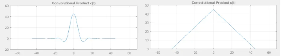
Figure 8: Approximation of the output of the different matched filters.
When comparing the 2 different outputs of the matched filters, it can be seen that there is less energy in the tails at the output of the RRC matched filter compared to the output of the 2-Path matched filter.
Transmitted signal
When comparing the transmitted signal of the situation using RRC filtering and the case where no technique is used, the only change is the message signal. The message signal is put through a RRC filter and because of this filter the square waves are turned into RRC’s. The RRC’s are then normalized and plotted together with the original message signal in figure 9. As seen in the figure less energy is captured in the tails after sending the message signal though a RRC filter. After this the new message signal is normalized, such that the
overall mean power still remains 1. After this normalization the bit energy calculations remain the same and no change has to be accounted for.
2.6 AWGN 2-Path Guard Interval
Apart from the RRC technique a guard interval is also considered. This guard interval implies that the overlap between 2 signals is compensated for, by changing a part of the symbol into zeros. This means that a part of the overlapping of the second arriving signal is zero, meaning less influence on the other signal is exerted.
Transmitted signal
The difference between the normal transmitted signal in equation 1 and the transmitted signal that is used now is at first only the change in the message signal. Instead of the NRZ BPSK message signal, now a message signal is sent where a certain length of the last part of each bit is replaced by zeros. The total bit time is called 𝑇𝑏 and the actual time the pulse is there is
called 𝑇𝑝, the difference between these two is the zero gap, which is called 𝑇𝑔. The cut
message signal is called 𝑚𝑔(𝑡). When cutting these bits without any extra thought, the mean
power of the message signal drops below 1 if taken over the entire bit time. The mean power however should be calculated over the pulse time, since 𝑃𝑦 should in this situation be defined
as 𝑃𝑦= 𝐸𝑏
[image:12.595.265.506.258.436.2]𝑇𝑝.
The general equation seen in equation 1 is changed into:
𝑦(𝑡) = 𝑥(𝑡) ∗ 𝑚𝑔(𝑡) ∗ cos(𝜔𝑟𝑡) + 𝑥(𝑡) (4)
𝑚𝑔(𝑡) = {𝑏0,0,
0 < 𝑡 < 𝑇𝑝
𝑇𝑝< 𝑡 < 𝑇𝑏
Where 𝑏0 is either 1 or -1.
Looking at this equation it can be seen that the intended zero part of the signal is not zero yet. This is because the spread signal is added to the multiplication and therefore also added to the zero part. Therefore 𝑥(𝑡) is also limited to have the zero part actually zero and not waste power.
Bit Energy Calculation
Since the transmitted signal is changed such that the power of the signal is different than in the normal case, a new theoretical mean power is derived. The bit energy is calculated as follows.
𝑦(𝑡) = 𝑥(𝑡) ∗ 𝑚𝑔(𝑡) ∗ cos(𝜔𝑟𝑡) + 𝑥(𝑡) ∗ 𝑐
Where the c implies the possible compensation that has to be done, which is already a division by √2 for optimal energy distribution; and 𝑥(𝑡) is limited.
𝐸𝑏 = 𝐸 [ ∫ 𝑦2(𝑡)𝑑𝑡
𝑘+𝑇𝑏
𝑘
]
𝐸𝑏 = 𝑃𝑥 ∫
1
2𝑚𝑔
2(𝑡) +1
2𝑚𝑔
2(𝑡) cos(2𝜔
𝑟𝑡) + 2c𝑚𝑔(𝑡) cos(𝜔𝑟𝑡) + 𝑐2𝑑𝑡
𝑘+𝑇𝑝
𝑘
=1
2𝑃𝑥 ∫ 1 𝑑𝑡
𝑘+𝑇𝑝
𝑘
+ 𝑃𝑥 ∫
1
2cos(2𝜔𝑟𝑡) + 2𝑐𝑏0cos(𝜔𝑟𝑡) 𝑑𝑡 + 𝑃𝑥∫ 𝑐
2𝑑𝑡
𝑘+𝑇𝑝
𝑘
𝑘+𝑇𝑝
𝑘
Where the second integral turns to zero if 𝜔𝑟 is a multiple of 2𝜋
𝑇𝑝 giving,
=1
2𝑃𝑥𝑇𝑝+ 𝑃𝑥𝑇𝑝𝑐
2
𝐸𝑏 = 𝑃𝑥(
1
2𝑇𝑝+ 𝑇𝑝𝑐
2)
Where if 𝑐 𝑟𝑒𝑚𝑎𝑖𝑛𝑠 √12 both parts have equal energy,
And since,
𝑃𝑦=
𝐸𝑏
𝑇𝑝
= 𝑃𝑥(
1 2+
1 2)
Giving,
𝑃𝑥= 𝑃𝑦
To maintain orthogonality between the spread signal and the information signal over one pulse interval, we chose the frequency offset as a multiple of 𝑇𝑝 instead of 𝑇𝑏. However, since
IDF filtering is done over𝑇1
𝑏, there will be added noise. One could argue about the choice of an IDF filter over 1
of the overlapping of the second signal is not captured. A lot of trade-offs can be taken into account for whether choosing 1
𝑇𝑝 or
1 𝑇𝑏.
2.7 AWGN Multipath
To check the actual effect of the ISI prevention techniques in a multipath, a multipath channel is described. As stated before, the multipath channel is described by a standard representation which is a TDL model, where the complex equivalent baseband channel has an impulse response
ℎ(𝑡) = ∑ ℎ𝑘𝛿(𝑡 − 𝑘∆𝜏), 𝐾
𝑘=1
Here, ℎ𝑘 serves as the resolvable channel tap coefficient; 𝛿(𝑡)is the Dirac delta function; ∆𝜏
is the spacing between consecutive taps and chosen as𝑓𝑠1; and K is the number of taps.
It is assumed that the tap variance 𝐸[|ℎ𝑘|2] decays exponentially with delay, i.e., the channel
follows an exponential power delay profile (PDP) [2].
𝑃ℎ(𝜏) =
𝑃ℎ
𝜏𝑟𝑚𝑠
exp (− 𝜏 𝜏𝑟𝑚𝑠
) , 𝜏 ≥ 0
(5)
Where 𝑃ℎis the total power gain of the channel and 𝜏𝑟𝑚𝑠 is the root-mean-square delay
spread. An approximation of the PDP for the time-discrete channel is
𝐸[|ℎ𝑘|2] ≅ 𝐶𝑒 −𝜏𝑘∆𝜏
𝑟𝑚𝑠, 𝑘 ≥ 1 (6)
Where C is a constant which ensures that the sum is equal to 1.
K can be calculated with the equation
𝐾 = −𝜏𝑟𝑚𝑠ln(𝐴) ∆𝜏
Where A is 10−2 (-20 dB) keeping the collective power in the taps to about 99%.
Channel coefficients
For a more practical analysis, the tap coefficients should be described as complex Gaussian distributed variables. For now however, the resolvable tap coefficients are chosen to be the root mean square of the channel taps strength. Where the average strength of the channel is dictated by the PDP. This gives
𝑐𝑘 = √𝐶𝑒 −𝜏𝑘∆𝜏
𝑟𝑚𝑠 (7)
This approach is chosen to get an easier insight on the influence of ISI in a general multipath. If the actual complex Gaussian distributed variables were to be used, a lot more research had to be done. Given the time frame in which this study is done, this is for now neglected.
Future problems
Because ∆𝜏 is 1
𝑓𝑠 and 𝑓𝑠 is chosen as close to 𝐵𝑥 but not exactly, an earlier stated problem
arises, implying that 𝑅𝑦(∆𝜏) ≠ 0. This will be further elaborated on in the experimental
2.8 AWGN Multipath Root Raised Cosine
The RRC technique, already mentioned in the AWGN 2-Path, is now implemented into the multipath. The same pulse shaping used in the 2-path can be integrated into the multipath. The only difference between the 2 systems is the description of the channel, which is already described in the section above.
2.9 AWGN Multipath Guard Interval
3. Experimental procedure and results
For a better understanding of the system, a simple implementation was created. This meant that an, already existing, scenario was used and further adapted. The existing scenario represented a simulation of NFOM in an AWGN channel. This scenario was then further adapted into a 2-path channel. Later this 2-path was again further adapted into, first a 2-path using pulse shaping and secondly, a 2-path which makes use of a guard interval.
3.1 AWGN
In the existing scenario the bit BER is calculated by comparing the input bit stream, which consists of 1000 bits, with the normalized output of the IDF. The IDF looks at one bit time, integrates over this bit time and gives the resulting outcome. Whether this result of integration is positive of negative indicates whether the bit is seen as a 1 or a 0, respectively. This can be compared with a match filter. The only difference is the sampling time. With the IDF the value of the area beneath the signal over one bit time, is at the last sample of the bit time, looking at a match filter the sampling time would be in the middle of the bit time. To get a reliable result the code is repeated. This means that multiple bit streams are keep being transmitted, until at least 100 errors are found.
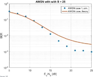
The BER is calculated for different values of 𝐸𝑏
𝑁𝑜 and then the BER of the simulation and the theoretical BER are plotted against the different values of 𝐸𝑏
𝑁𝑜 and a spreading factor of 25. A
graph of the result can be seen in figure 10. It can be seen that for the lower values of 𝐸𝑏
𝑁𝑜 the simulation case has a slightly worse performance compared to the theory. Considering the larger values of 𝐸𝑏
[image:16.595.93.471.449.764.2]𝑁𝑜 it can be seen however that the results show a better performance than the theory. This can be explained by assumptions that are made in the theoretical analysis
3.2 Reliability of BER
As mentioned before, every simulations runs until more than 100 errors are found. This is a lot better than stopping after the first error found. It still is not perfect however. Also because the message signals are generated randomly, small changes could appear. When comparing different simulations with each other it should be taken into account that minor changes could have appeared through the difference in their message signals, since this is generated randomly for every simulation. To actually be able to compare the different techniques perfectly separate sections are made to compare them. This is done by creating one code using where all techniques are applied. This way one message signal is created and used, and differences in results are caused by the techniques used and not the difference in message signals.
3.3 AWGN 2-path
After the general understanding of the AWGN scenario, this scenario was further adapted to represent a 2-path channel. This was done to see what influence a 2-path would have on the BER.
In the simulation a ratio of 80% of the amplitudes, between the first arriving signal and the second arriving signal, is chosen. The delay between the paths is chosen to be around 10% of one bit time. This is realized by choosing a certain value of samples that represent the delay. The sampling frequency influences the number of samples per bit time. A given bit time of
𝑇𝑏 = 5 𝜇𝑠 and a sampling frequency of fs = 15 𝑀𝐻𝑧 give 75 samples per bit time. The
sampling frequency should be at least twice the bandwidth, to prevent aliasing. As seen before, a restriction was given on the time delay since the autocorrelation 𝑅𝑦(𝑇𝑑) should
equal zero. The delay should keep this restriction and is kept when a value around 10% of the bit time is chosen.
To really check the influence of 𝑅𝑦(𝑇𝑑), a significant small delay is chosen such that 𝑅𝑦(𝑇𝑑)
has a value which significantly influences the power. If then the theoretic power 𝑃𝑦 is
compared with 𝐸[|𝑦𝑡𝑟𝑎𝑛𝑠(𝑡)|2 ], where 𝑦𝑡𝑟𝑎𝑛𝑠(𝑡) = 𝑦(𝑡) ∗ ℎ(𝑡) which represents the
separate signals added up, a difference is found. This difference can be assigned to 𝑅𝑦(𝑇𝑑)
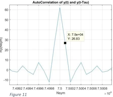
not being equal to zero. For a specific case, where the delay is chosen small, the following values are found
𝑃𝑦= 63,24 𝑎𝑛𝑑 𝐸[|𝑦𝑡𝑟𝑎𝑛𝑠(𝑡)|2 ] = 88,19
This difference then seems to come from 𝑅𝑦(𝑇𝑑) not being equal to zero.
To check this the autocorrelation is plotted and can be seen in figure 11. This difference is not the exact same as the value that is found in the figure, but this is because of the term 2𝑐1𝑐2that
[image:17.595.281.505.575.768.2]arises in front of the autocorrelation and the fact that the graph should follow a smooth sinc function. The however could not be realised in the simulations. The graph does show that the difference is caused by the autocorrelation.
Future problems
Due to the characteristics of the channel, as mentioned before, the delay should be chosen such that 𝜏𝑑=
1
2𝐵𝑥 or higher, since the first zero crossing is at 1
2𝐵𝑥 . Later in the multipath
channel it is seen however that this case cannot be realized correctly in simulation.
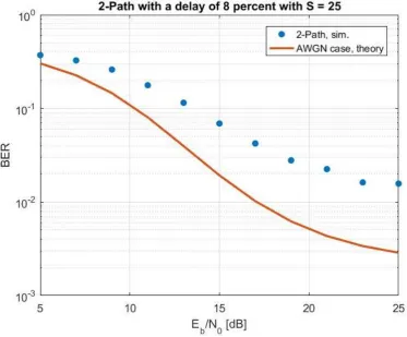
Simulation
[image:18.595.93.467.203.512.2]A simulation with a delay of 8% of one bit time is done while taking into account the previous findings and is shown in the following figure.
It can be clearly seen that the BER has increased compared to the normal AWGN case. To do an extra check whether this increase of the BER is actually caused by ISI, a worst case scenario is considered. When 2 ones are next to each other they don’t negatively influence each other, this is the same case when 2 zeros are next to each other. When however a 1 and a 0 are next to each other, the first bit does negatively influence the second one. This means that a worst case scenario would be a message signal with only switching bits which is represented by
𝑚(𝑡) = [1010 … 1010] .
[image:19.595.96.472.254.571.2]If the case using a random message signal is plotted above the worst case scenario it shows that something else is influencing the signal. If it is between the worst case scenario and the theory the results are more reliable. In figure 13 it can be seen that the case using a random message signal falls between the worst case scenario and the theory:
Figure 13
3.4 AWGN 2-path Root Raised Cosine Pulse Shaping
To try and increase the performance of the system by compensating the detrimental effect of ISI, RRC pulse shaping is used.
Figure 14
3.5 AWGN 2-Path Guard Interval
After simulating the pulse shaping another approach was considered. Keeping in mind that the signals only have about 10% as a maximum delay, this gap could be easily bridged by replacing the last part of a bit time with zeros. For this reason a simulation is done were the last part of each bit is replaced by zeros. The following result where found with a delay of 8% of a bit time and a guard interval of equal length.
[image:20.595.93.440.470.761.2]Looking at the graph it can be clearly seen that a much better performance is achieved when using the guard interval technique compared to the normal case and the RRC case.
After several simulations it turned out that with different delays, different guard intervals gave the most optimal result. In this study a certain, decent, value for the guard interval is chosen and this development is not further studied. It was also shown that with delays above 20% the effect of the Guard Interval significantly drops and the technique does not increase the performance anymore, this should be taken into account when working towards the multipath channel.
3.6 Comparison of the different techniques on the 2-path
[image:21.595.95.452.271.579.2]To get a better comparison of the normal case, RRC technique and the guard interval technique the different situations are combined into one code. In this code the same random message signal is used. In figure 16 the results can be seen.
Figure 16
From looking at the figure it clearly shows that at high values for𝐸𝑏
𝑁𝑜, both the RRC and the guard interval technique show promising results. Whether these techniques actually increase the performance when considering a general multipath is still unknown. This is simulated in further sections.
To check the influences of the techniques on the worst case scenarios, this case is also simulated and can be seen in figure 17. In this simulation a message signal is used which is represented by (𝑡) = [1010 … 1010] .
Figure 17
3.7 AWGN Multipath
Instead of just simulating a simple 2-path, a general multipath channel situation is simulated. To represent the correct multipath an approximation of an exponential PDP is chosen to create the correct resolvable taps, 𝑐𝑘 which is already stated in the theory. In this simulation
they are not yet represented as independent, zero-mean complex Gaussian variables but just deterministic taps that are following an exponential curve.
For this situation, as mentioned before, a TDL model is used. This is done by using an existing approximation of the PDP, equation 6. Then equation 7 is used to create the coefficients that need to be in front of the different delayed signals. Then ℎ(𝑡) is convolved with 𝑦(𝑡), where
𝑦(𝑡) = 𝑥(𝑡) ∗ 𝑚(𝑡) ∗ cos(𝜔𝑟𝑡) + 𝑥(𝑡), to create one signal which are all the different
multitaps combined. At the receiver side the same situation still exists which is already presented with the 2-path.
A problem that arose was, the previously mentioned fact, that 𝑅𝑦(∆𝜏) ≠ 0. This presence was
checked in the same way as it was done with the 2-path. A quick look at some calculations already show this presence, since ∆𝜏 was chosen equal to 𝑓𝑠1 which means that the delay would equal 1 sample time. 𝑓𝑠
is however not exactly equal to 2𝐵𝑥
but a bit higher, say 2.4𝐵𝑥. This means that ∆𝜏 = 1
2.4𝐵𝑥 which is
smaller than 2𝐵𝑥1 which makes
𝑅𝑦(∆𝜏) ≠ 0. To make 𝑅𝑦(∆𝜏) = 0
however one could choose ∆𝜏 = 2𝐵𝑥1 instead of𝑓𝑠1 . The simulation however is limited by the sampling frequency, 𝑓𝑠, meaning that between samples no points can be found. This gives the restriction that ∆𝜏, as a number of samples, has to be rounded to the closest integer value. For ∆𝜏 = 1
2𝐵𝑥 this means ∆𝜏 = 1.2 𝑠𝑎𝑚𝑝𝑙𝑒𝑠 which is rounded to 1 sample which makes no
difference in the point where 𝑅𝑦(∆𝜏) is checked. The problem is visualized in figure 18. This
could not be accounted for which means that some of the assumptions made in the theory cannot be fulfilled.
Because theory says that 2𝐵𝑥1 is the first zero crossing this is indicated in the graph as the actual first zero crossing. The actual value of 2𝐵𝑥1 is however a bit to the left. This is caused by the imperfection that is the result of the limited samples. This is clearly seen by comparing this figure with figure 7, which was the smooth sinc function. Optimally the graph would follow the smooth curve shown in that figure. It can now be clearly seen that, because the figure is not smooth and it is between 2 samples, the first zero crossing cannot be achieved.
[image:23.595.92.504.260.558.2]Results
The result of a simulation of the TR system in a multipath with 𝜏𝑟𝑚𝑠 = 200 𝑛𝑠, which
[image:24.595.95.405.134.396.2]represents a certain environment, can be seen in figure 19.
Figure 19
In the graph it can be clearly seen that at this value for 𝜏𝑟𝑚𝑠 the BER has increased a lot
compared to the AWGN case where no ISI was involved.
For a better view of the influence of different values of 𝜏𝑟𝑚𝑠 a plot is made for different values
of 𝜏𝑟𝑚𝑠 and for one 𝐸𝑏
𝑁𝑜, in this case 25 dB. This is shown in figure 20.
[image:24.595.90.423.489.761.2]This graph shows that, as expected, at higher 𝜏𝑟𝑚𝑠 the BER increases. This increase is expected
because, for higher values of 𝜏𝑟𝑚𝑠 K increases, which means there are more taps and
therefore more signals arriving with a greater delay. This graph is also plotted for the 2 techniques in the next chapters to see whether or not this performance can be increased and for what 𝜏𝑟𝑚𝑠 they improve the performance the most.
3.8 AWGN Multipath Root Raised Cosine
A TR system using the RRC technique in a multipath with 𝜏𝑟𝑚𝑠 = 200 𝑛𝑠 is simulated. This
[image:25.595.95.406.241.500.2]simulation was created by combining the multipath scenario with the RRC technique. The result of this simulation can be seen in figure 21.
Figure 21
It seems that this figure shows better results than figure 19. This is however only for this specific value of 𝜏𝑟𝑚𝑠. To actually show whether the technique improves the BER for different
environments, the BER is plotted against different values of 𝜏𝑟𝑚𝑠in the following figure. The
Figure 22
3.9 AWGN Multipath Guard Interval
A TR system using the guard interval technique in a multipath with 𝜏𝑟𝑚𝑠= 200 𝑛𝑠 is
simulated. This simulation was created by combining the multipath scenario with the guard interval technique. The result of this simulation can be seen in figure 23. A big difference with the previous results can be seen at high values of 𝜏𝑟𝑚𝑠. It was also seen again, after several
simulations, that at different values for 𝜏𝑟𝑚𝑠, different guard intervals were most optimal.
[image:26.595.94.415.460.737.2]The results of the simulation, when using a guard interval, seem a lot more promising than when using the RRC technique. For this specific value of 𝜏𝑟𝑚𝑠, several BER’s are found which
are even better than the AWGN theory case. These are found at high values of𝐸𝑁𝑏
𝑜, which seems to show the guard interval is most optimal here.
For this technique the BER of a certain value of 𝐸𝑏
𝑁𝑜 is plotted against several values of 𝜏𝑟𝑚𝑠.
[image:27.595.95.424.187.457.2]This can be seen in figure 24.
3.10 Comparison of the different techniques on the multipath
The different results of the different techniques, in a multipath channel, are plotted into one graph seen in figure 25. In this graph it can be clearly seen that the guard interval technique shows better results for the lower values of 𝜏𝑟𝑚𝑠. The RRC technique however, shows no
[image:28.595.93.422.184.466.2]better performance whatsoever compared to the general multipath situation. No actual reason can be found why the RRC does seem to work in the 2-path, but not in the multipath. Several changes were made to the characteristics of the RRC filter, but without any success.
4. Evaluations
4.1 Conclusion
A previous study was done on an N-FOM technique in multipath channels. In certain environments, the system performance degraded due to ISI. In this report, we looked at ISI in the N-FOM and 2 potential ISI-prevention techniques.
The 2 ISI prevention techniques that were looked further into were the RRC and guard interval techniques. We first looked at a simple 2-path channel model. It turns out that in this 2-path channel model both the RRC and the guard interval technique show a promising improvement in performance. At relatively high delays the guard interval starts to be less effective and even worsening the results at a certain high delay when compared to the case where no ISI prevention technique is used. Using the RRC gives a better performance than the 2-path channel model were no ISI prevention technique is used. At low delays a slightly worse performance is achieved when compared to the guard interval technique. At higher delays the RRC goes towards the normal case and stays there.
We then further extended the channel model to a general multipath. The channel coefficients were chosen to be the root mean square of the channel tap strength. This means that the channel is considered deterministic. The average strength of the channel taps is dictated by the power delay profile. This choice for deterministic channel taps was made, to get an actual simulation of a multipath within the given time constraint.
For the guard interval technique the better performance, that was seen in the 2-path, is also true for the multipath, however instead of again looking at a certain delay, the delay spread is considered. It also turned out that at different values for 𝜏𝑟𝑚𝑠 different guard intervals
resulted in the most optimal results.
When looking at the RRC technique in the multipath it was found that it did not influence the performance as anticipated, because no increase in performance was found. Also no change in the results were found when changing certain characteristics of the RRC filter. It is possible that these found results emerge from other unknown effects. To check these other unknown effects in the actual multipath one should first check whether the RRC is implemented in the right way in the 2-path. From the perspective of this study it seems that the RRC technique is implemented in the right way, but the multipath RRC does not show the results that are expected. This means a discrepancy emerged when going from the 2-Path RRC to the multipath RRC.
4.2 Recommendation
As mentioned before, the optimal guard interval for different environments was not yet found. This optimum could be studied and fully tested in further research to increase the already satisfying result resulting from the guard interval.
To actually check the reason why the RRC does not seem to work in the multipath a further study could be done. This is important, since at first glance, in the 2-path, the technique seems to work. One could use a certain value of 𝜏𝑟𝑚𝑠, which causes the multipath to act as a 2-path.
Only the 2 mentioned techniques were looked into for reasons mentioned before, however one could also look into several other techniques such as changing the modulation technique, maximum-likelihood sequence estimation and equalizers, when given more time and the freedom to make changes in the architecture of the communication scheme. This could result into an even better performance in the system than using the guard interval.