Brain network analysis : separating cost from topology using cost integration

University of Warwick institutional repository: http://go.warwick.ac.uk/wrap

This paper is made available online in accordance with

publisher policies. Please scroll down to view the document

itself. Please refer to the repository record for this item and our

policy information available from the repository home page for

further information.

To see the final version of this paper please visit the publisher’s website.

Access to the published version may require a subscription.

Author(s): Cedric E. Ginestet, Thomas E. Nichols, Ed T. Bullmore and

Andrew Simmons

Article Title: Brain Network Analysis: Separating Cost from Topology

Using Cost-Integration

Year of publication: 2011

Link to published article:

http://dx.doi.org/10.1371/journal.pone.0021570

Publisher statement: Citation: Ginestet CE, Nichols TE, Bullmore ET,

Simmons A (2011) Brain Network Analysis: Separating Cost from

Topology Using Cost-Integration. PLoS ONE 6(7): e21570.

doi:10.1371/journal.pone.0021570

Using Cost-Integration

Cedric E. Ginestet1,2*, Thomas E. Nichols3, Ed T. Bullmore4, Andrew Simmons1,2

1Department of Neuroimaging, Institute of Psychiatry, King’s College London, London, United Kingdom,2National Institute of Health Research (NIHR) Biomedical Research Centre for Mental Health, Institute of Psychiatry, King’s College London, London, United Kingdom,3Department of Statistics, University of Warwick, Coventry, United Kingdom,4Brain Mapping Unit, Department of Psychiatry, School of Clinical Medicine, University of Cambridge, Cambridge, United Kingdom

Abstract

A statistically principled way of conducting brain network analysis is still lacking. Comparison of different populations of brain networks is hard because topology is inherently dependent on wiring cost, where cost is defined as the number of edges in an unweighted graph. In this paper, we evaluate the benefits and limitations associated with using cost-integrated topological metrics. Our focus is on comparing populations of weighted undirected graphs that differ in mean association weight, using global efficiency. Our key result shows that integrating over cost is equivalent to controlling for any monotonic transformation of the weight set of a weighted graph. That is, when integrating over cost, we eliminate the differences in topology that may be due to a monotonic transformation of the weight set. Our result holds for any unweighted topological measure, and for any choice of distribution over cost levels. Cost-integration is therefore helpful in disentangling differences in cost from differences in topology. By contrast, we show that the use of the weighted version of a topological metric is generally not a valid approach to this problem. Indeed, we prove that, under weak conditions, the use of the weighted version of global efficiency is equivalent to simply comparing weighted costs. Thus, we recommend the reporting of (i) differences in weighted costs and (ii) differences in cost-integrated topological measures with respect to different distributions over the cost domain. We demonstrate the application of these techniques in a re-analysis of an fMRI working memory task. We also provide a Monte Carlo method for approximating cost-integrated topological measures. Finally, we discuss the limitations of integrating topology over cost, which may pose problems when some weights are zero, when multiplicities exist in the ranks of the weights, and when one expects subtle cost-dependent topological differences, which could be masked by cost-integration.

Citation:Ginestet CE, Nichols TE, Bullmore ET, Simmons A (2011) Brain Network Analysis: Separating Cost from Topology Using Cost-Integration. PLoS ONE 6(7): e21570. doi:10.1371/journal.pone.0021570

Editor:Olaf Sporns, Indiana University, United States of America

ReceivedDecember 14, 2010;AcceptedJune 4, 2011;PublishedJuly 28, 2011

Copyright:ß2011 Ginestet et al. This is an open-access article distributed under the terms of the Creative Commons Attribution License, which permits unrestricted use, distribution, and reproduction in any medium, provided the original author and source are credited.

Funding:CEG and AS were supported by a fellowship from the United Kingdom National Institute for Health Research (NIHR) Biomedical Research Centre for Mental Health (BRC-MH) at the South London and Maudsley NHS Foundation Trust and King’s College London. This work has also been funded by the Guy’s and St Thomas’ Charitable Foundation as well as the South London and Maudsley Trustees. The funders had no role in study design, data collection and analysis, decision to publish, or preparation of the manuscript.

Competing Interests:The authors have declared that no competing interests exist. * E-mail: [email protected]

Introduction

In the last decade, the biological and physical sciences have witnessed a proliferation of publications adopting a network approach to a wide range of questions. This interest in networks was originally stimulated by the seminal works of Watts et al. [1] and Barabasi et al. [2], who introduced the concepts of small-world and scale-free networks, respectively. Some of these ideas have been adopted in neuroscience at both a theoretical [3,4] and experimental level [5]. Most of the research in this area has attempted to classify the topology of brain networks based on anatomical or functional data [6–8].

A question that naturally arises from such applications of graph theory is whether or not the topological properties of these brain networks are stable across different populations of subjects or across different cognitive and behavioral tasks. A common hypothesis that neuroscientists may wish to test is whether the small-world properties of a given brain network are conserved when comparing patients and healthy controls. Bassett et al. [9], for example, have studied differences in anatomical brain networks

between healthy controls and patients with schizophrenia. Other authors have evaluated whether the topological properties of functional networks vary with different behavioral tasks [10–13]. The properties of brain network topology have also been studied at different spatial scales [14] and using different modalities, such as EEG [15,16], and fMRI [6,7]. There is therefore considerable interest in comparing populations of networks –which may represent different groups of subjects, several conditions of an experiment, or the use of different levels of spatial or temporal resolution. We note that such research questions are more likely to arise when subject-specific networks can be directly constructed. This has been done in the context of both functional and structural MRI [17,18].

metrics used to compare networks are sensitive to differences in these graphs’ number of edges. Drawing comparisons on the sole basis of topology therefore requires some level of control of cost discrepancies between these network populations. Secondly, this issue is compounded by the fundamental division between weighted and unweighted graphs. The problem of disentangling differences in connectivity strength from topological differences therefore needs to be resolved in a distinct manner depending on whether weighted or unweighted graphs are being considered. The focus, in this paper, will be on weighted networks since these are more likely to be found in the biomedical sciences than their unweighted counterparts.

Historically, however, network analyses have concentrated on unweighted graphs. The application of graph theory to biological and artificial networks was originally motivated by the discrete nature of the problems of interest. Both Watts et al. [1] and Barabasi et al. [2] mainly considered binary relations between sets of elements, which readily produced adjacency matrices that could then be used to construct unweighted graphs. Watts et al. [1] matched some networks of interest with their random and regular equivalents. In their case, the matching procedure ensured that both random and regular networks possessed the same total number of nodes and edges as the original graph. Current practice in MRI-based neuroscience and other biomedical applications, however, tends to produceweightedconnectivity networks. This is because MRI data take values on a continuous scale, which lends itself to the application of real-valued measures of association, such as the correlation coefficient or the synchronization likelihood among others. While different populations of unweighted networks can readily be compared by matching each network with a random network possessing an identical number of edges; there is, as yet, no consensus on how to compare populations of weighted networks in a systematic manner.

This problem can be illustrated with a straightforward example. In panel (a) of Figure 1, a pair of weighted networks are represented by their correlation matrices. We are interested in comparing the topology of the corresponding weighted graphs. Since these networks differ in their mean correlation coefficients, a simple thresholding of these matrices will produce graphs of different wiring costs, i.e. different number of edges. Naturally, this thresholding is only one of the possible thresholding approaches that could be adopted. This non-uniqueness is due to the fact that graph topology is expressed in the language of discrete mathematics, whereas correlation coefficients are real-valued functions. That is, one cannot directly adopt concepts originally developed for unweighted graphs for the analysis of weighted graphs.

In this paper, we consider two main approaches to the problem of weighted network comparison. Firstly, following other authors, we evaluate the use of weighted topological metrics, which are weighted equivalents of graph-theoretical metrics for unweighted networks [19,20]. Secondly, we consider the utilization of cost-integrated measures of topology, where all the possible wiring costs of a network are taken into account. When unweighted, a graph’s wiring cost is defined as its number of edges. Integrating over wiring cost can here be interpreted in statistical terms, as an analog to the Bayesian integration of nuisance parameters. Doing so, we are averaging out the ‘uncertainty’ in the choice of a particular level of cost. Cost-integrated topological measures have been popular in the neuroscientific literature [6,21]. However, different authors have chosen different integration intervals. We therefore explore the consequences of integrating a topological metric with respect to different subsets of the cost interval.

Note that our approach substantially differs from the one adopted by Wijk et al. [22], who proposed several formulas relating cost levels and topological measures, such as the characteristic path length or the clustering coefficient. Instead, in this paper, we are concerned with formally deriving what is the effect of integrating a particular topological measures over cost levels, in order to assess whether this is a successful manner of disentangling differences in cost from differences in topology. In particular, although Wijk et al. [22] reviews several ways of controlling for differences in cost, they do not consider cost-integration, per se. This paper can therefore be seen as a contribution to the literature on weighted network analysis, where we formally clarify the utilization of cost-integration when comparing topological metrics.

The concept of topology in the context of this paper will be defined in a quantitative manner. This should be contrasted with the qualitative definition adopted by previous authors. Wijk et al. [22], for instance, assume that networks that represent different realizations of the same ‘generative model’ should be regarded as topologically identical. Indeed, several realizations of an Erdo¨s-Re´nyi model with fixed edge probability share a common generative model and therefore can be said to have an identical topology. In practice, however, such a generative model is unknown. Thus, we will refer to this type of classification as a topological taxon. A taxonony of commonly encountered networks may include the random topology of the Erdo¨s-Re´nyi model, the regular lattice and the small-world topology among others. Such a nomenclature is qualitative because it relies on discrete categories. By contrast, we wish to adopt a quantitative perspective on this problem, whereby topology is operationalized in terms of specific topological properties such as the clustering coefficient (CC), for instance. In this perspective, two Erdo¨s-Re´nyi models with identical edge probability may display different levels of global and local efficiencies and will therefore be considered to have distinct topological properties. Therefore, we distinguish between a qualitative approach based on topological taxonony and a quantitative approach based on topological properties. Given that generative models are latent, our quantitative definition of topology appears better suited to the empirical study and comparison of complex networks.

The above definition of network topology, however, assumes that the networks under comparison have identical numbers of vertices and edges. When this is not the case, or when one is comparing two populations of weighted networks, the question of whether or not these networks have similar topological properties becomes arduous. Our main aim, in this paper, is therefore to identify the situations within which one can safely conclude that different weighted networks share the same topological properties. In particular, we explore whether cost-integration answers this problem. Specifically, we consider whether cost-integration is a useful way of disentangling weighted cost from topology.

discuss the findings of this paper in light of the current utilization of networks in the biomedical sciences. Finally, we close with a set of recommendations on how to conduct weighted network analysis in practice and how to report the findings arising from this type of research. An R package entitled NetworkAnalysis (http://CRAN.R-project.org/package = NetworkAnalysis) has been developed that makes available the methods discussed in this paper.

Results

Network Types and Topologies

Unweighted, Weighted and Fully Weighted Networks. For clarity of exposition and consistency with the previous literature, we will here employ the notation used by Kolaczyk [23]. A comprehensive introduction to the theory of complex networks can be found in Newman [24]. In the following, the terms metrics and measures will be used interchangeably to refer to a function quantifying the topological structure of a network. Our use of the terms metric and measure is unrelated to the mathematical definitions of these concepts in topology and measure theory, respectively. Similarly, we here utilize the graph-theoretical

definition of the term cost, which is not related to its use in a probabilistic setting.

An unweighted undirected graph or network G is formally defined as an ordered pair(V,E), whereVis a set of vertices, points or nodes, andE is a set of edges or connections linking pairs of nodes. ThereforeE(V6_{V, where} 6 _{is the Cartesian product.}

The cardinality –i.e. the number of elements– ofVandEwill be referred to asNV:~jVjand NE:~jEj, respectively, wherej:j

denotes the number of elements in a set, and:~ _{that the} left-hand-side is defined as the right-left-hand-side. Moreover, the terms network and graph will be used interchangeably. A graph with the maximal number of edges is referred to as a complete or saturated graph. For a given network G, we denote the corresponding saturated graph asGSat_{. The cardinality of the edge set ofG}Sat_is

denoted byNI to distinguish it fromNE. Here, the setI(G), for

any graphGis the set of indices of all possible edges inG. That is,

I(G):~_f(i,j):1ƒivjƒN_Vg: ð1Þ

This notation for the set of indices of all possible edges inGwill be useful when describing the topology of G based on its shortest paths.

Weighted undirected graphs will be denoted by the triple G:~(V,E,W), whereW(G) is a set of weights, whose elements are indexed by the entries inE(G), such that

w_ei~w_vjvh, ð2Þ

for some edgeei:~vjvh. Thus, every weighted undirected graph

will necessarily satisfy

NE~NWƒN_I, ð3Þ

where NW:~jW(G)j. The weight set populates a symmetric

matrixW, whose diagonal elements are null. Graphs that satisfy NW~NI will be referred to asfully weighted graphs. Note that, in

general, we will not draw an explicit difference between a weighted and an unweighted network through our notation. However, which one we are referring to should be understandable from the context.

There are a wide range of different weighted measures of internodal association. Our methodological development, in this paper, applies to any choice of association metric. This includes correlation coefficients, partial correlations, synchronization likelihoods and others. For simplicity, we will assume that the association weights, wij’s, lie in the unit interval,½0,1. Roughly,

these standardized weights,wij, can be interpreted as the strength

of the association between nodes i and j, with larger values indicating a greater level of association. Such standardization can be obtained straightforwardly, in practice. For the case of the Pearson’s correlation coefficientrij, for example, the standardized

weights can be defined as,

wij:~1{ 1{rij

2

: ð4Þ

Note that the use of standardized correlation coefficients suffers from two potential pitfalls. Firstly, since negative correlations are transformed into positive measures of association, it follows that we are amalgamating different subsets of edges, which may play very different roles. That is, while subnetworks of negatively correlated vertices may reflect inhibitory processes, subnetworks of positively correlated vertices may reflect excitatory processes. Secondly, since pairs of vertices linked by a small amount of correlation, either positive or negative, will be transformed to take a value close to0:5; it follows that we may be introducing a spurious amount of random noise in such a weighted network analysis, as correlation coefficients close to zero are likely to be non-significant. Our approach to weighted network analysis in this paper, however, centres on thresholding the weighted networks of interest and therefore does not explicitly take into account the direction of the association. Moreover, our focus will be on fully weighted networks, such as a standardized correlation matrix, where all entries are greater than 0. Therefore, in the sequel, Gwill refer to a fully weighted graph, except when specified otherwise. We will discuss the use and limitations of cost-integration for non-fully weighted graphs in the discussion.

Classical Measures of Network Topology. A wide range of network topological metrics have been proposed in the literature [20]. Two types of measures are generally of interest, which are sometimes referred to as (i) integration metrics and (ii) specialization metrics. The former category of topological measures quantifies a network’s capacity to transfer information globally, whereas the latter reflects a network’s capacity to transfer

information locally. This distinction originated with the work of Watts et al. [1], who considered the characteristic path length (CPL), on one hand, and the clustering coefficient (CC), on the other hand, as measures of global and local information transfer, respectively. Although these metrics have been successfully used in a wide range of settings, Latora et al. [19] have introduced two analog metrics: the global and local efficiencies, which will be more useful in our context. These two measures retain the interpretation of the CPL and CC, while being applicable to a wider range of networks. Specifically, the global efficiency metric can be computed for any network, irrespective of its level of sparsity, which is not true for CPL. That is, the CPL becomes infinite when a graph is disconnected [25]. By contrast, the global efficiency is well-defined for any networks. For consistency, we will therefore use the global and local efficiencies to characterize global and local transfer of information in brain networks, respectively. Note, however, that analogously to the CC, the local efficiency is undefined for networks that contain isolated nodes. Thus, we set the efficiency of an isolated node to zero, which allows to integrate local efficiency over the full range of costs.

One of the remarkable aspects of global and local efficiencies is that they can both be subsumed under the general concept of information transfer efficiency, which is defined for any unweight-ed graphG~(V,E)–connected or disconnected– as [19],

E(G):~ 1

NV(NV{1) XNV

i~1 XNV

j=i

d{1 ij ~

1

NI X

I(G)

d{1 ij , ð5Þ

where the summation over the setI(G) is over all the pairs of indices(i,j)as in equation (1), and dij denotes the length of the

shortest path between verticesiandjin the adjacency matrix ofG, with dij:~? when these two nodes are not connected. The

summation over j=i includes all indices between 1 and NV

different fromi. The global and local efficiencies of networkGare then readily derived from equation (5), such that

EGlo_{(G):~E(G), and E}Loc_(G):~ 1

NV XNV

i~1

E(Gi), ð6Þ

whereGiis the subgraph ofGthat includes all the neighbors of the

ith _{node. That is,V(G}

i):~fvj[Gjvj*vig, where vj*visignifies

that nodes i and j are connected. By convention, we have vi=[V(Gi)[19,26]. Note that both global and local efficiencies are normalized quantities with values in the unit interval –that is E(G)[½0,1. The global efficiency of a graphGcan be interpreted as the average ‘speed’ of information transfer between any pair of nodes inG, with a high value ofEGlo_{(G)indicating a high average}

‘speed’, and therefore efficient information transfer. Similarly, the local efficiency of a graphG can be interpreted as the average global efficiency of theNV subgraphs ofG, where again a high

value forELoc_{(G) implies efficient local information transfer, on}

average.

applies to all topological metrics that can be computed for any level of sparsity. We will discuss the generalization of our results to other topological measures in the Discussion section.

Cost and Weighted Cost. In network analysis, it is often of interest to quantify the cost or wiring cost of an unweighted graph. In this section, we extend this concept to weighted networks. This generalized version of cost will be termed the weighted cost or weighted density.

The cost or density, K:~K(G), of an unweighted network G~(V,E)quantifies the relative number of connections inGas a proportion of the number of edges contained in theNV-matched

saturated networkGSat_{. That is,}

K(G):~ jE(G)j

jE(GSat_)j~

NE

NI

, ð7Þ

where NI:~NV(NV{1)=2. The computation of the cost of a

network G implicitly refers to the adjacency matrix A of that network. Hence, we can reformulate the definition in equation (7) by explicitly usingAas follows,

K(G)~

PNV i~1

PNV j=iaij PNV

i~1 PNV

j=iaSatij

~ 1

NI X

I(G)

aij, ð8Þ

where theaSat

ij ’s denote the elements of the adjacency matrixA Sat

, which represents a saturated network ofNV nodes.

Similarly, it will be of interest to quantify the cost of a weighted network, which will be referred to as KW(G). We define it by

generalizing the relationship between an unweighted graph and its adjacency matrix in order to apply it to weighted graphs and their association matrices. However, to extend the concept of cost to a real-valued association matrix, sayW, we need to formalize what we mean by asaturated weighted graph. A natural choice is to define WSatas a matrix of order(NV|NV)with unit entries. Formally,

WSat:~1(NV|NV). Using this saturated association matrix, we

can now define the cost of a weighted graph as follows,

KW(G):~ PNV

i~1 PNV

j=iwij PNV

i~1 PNV

j=iwSatij

~ 1

NI X

I(G)

wij, ð9Þ

where wSat

ij ’s are the elements of W Sat

. The non-standardized version of the cost of a weighted network in equation (9) was introduced by Fallani et al. [11]. Thus, the weighted cost of G~(V,E,W) is the mean of the off-diagonal elements in W, populated by the setW. This is reminiscent of our starting point in equation (7), where the same observation can be made about unweighted networks. In the sequel, the concept of weighted cost will be used interchangeably with the phrase connectivity strength. Note that depending upon which standardization one chooses, one may obtain different types of weighted costs. In particular, KW

could also be standardized with respect to the number of elements inW. This would produce a different measure. In this paper, we will assume that the networks under consideration are fully weighted, such thatNE~NW~NI, and therefore these two types

of weighted costs are equivalent.

There is currently no guidance in the literature on how to quantify the topological aspects of a weighted network. We review here two approaches to this problem in the following two sections: (i) weighted, and (ii) cost-integrated metrics of network topology. We describe and define these two families of measures, in turn.

Weighted Measures

A natural approach to the problem of quantifying the topology of weighted networks is to translate unweighted measures, such as efficiency metrics, for example, into a weighted format. This is a very general procedure, which has been introduced by several authors including Latora et al. [19] and Rubinov et al. [20]. Weighted versions of classical metrics commonly rely on the definition of a weighted shortest path. For unweighted networks, the shortest pathdijbetween nodesiandjinG~(V,E)is defined

as the following minimization,

dij:~ min

Pkl[P_ij(G)jE(Pkl)j, ð10Þ

wherePij(G)is the set of all paths between nodesiandjthat are

subgraphs of G. A subgraph Pij(G is a path if and only if

i,j[V(Pij)such that

E(Pij)~fia,ab,. . .,yz,zjg, ð11Þ

where each pair of letters stands for an edge. One can similarly define a weighted shortest path, dW

ij , for some weighted graph

G~(V,E,W)as follows,

dW

ij :~ min Pkl[P_ij(G)

X

uv[E(_Pkl)

f(wuv), ð12Þ

where the weighted edge set of a path now takes the form,

W(Pij)~ wia,wab,. . .,wyz,wzi

, ð13Þ

using the notational convention introduced in equation (2). Since we have normalized the association weights,wij’s, the real-valued

functionf(:)is restricted to a map of the formf :½0,1.½0,1. A convenient choice off(:)is the inverse function,f(wij):~1=wij.

It now suffices to use our chosen definition of the weighted shortest path dW

ij , in order to obtain a weighted version of the general

efficiency metric in equation (5), which gives

EW(G):~ 1

NV(NV{1) XNV

i~1 XNV

j=i 1 dW ij ~ 1 NI X I(G) 1 dW ij

: ð14Þ

Note that weighted efficiency is here bounded between0and1. Since the standardized association weights take values in½0,1, it then follows thatdW

ij §1, and therefore1=dijW[½0,1, for every pair

of vertices.

Cost-integrated Measures

A second approach to the problem of quantifying the topology of weighted networks proceeds by integrating the metric of interest with respect to cost. Here, some authors have integrated over a subset of the cost range [7], whereas others have integrated over the entire cost domain [27]. This second family of metrics will be referred to as cost-integrated measures. Given a weighted graph G~(V,E,W), the cost-integrated version of a topological metric T(:)is defined as follows,

Tp(G):~ X

k[V_K

T(c(G,k))p(k), ð15Þ

realizations in lower case, andp(k) denotes the probability mass function ofK. SinceK is discrete, it can only take a countably finite number of values, which is the following set,

VK:~ 1

NI , 2

NI

,. . .,NI{2

NI

,NI{1

NI , 1:0

~:k, ð16Þ

where, as before,NI:~NV(NV{1)=2~jVKj. It will be useful to

treatVKas an ordered set,k, whose elements,kt’s, are arranged in

increasing order and indexed by t~1,. . .,NI. The function

c(G,k)in equation (15) is a thresholding function, which takes a weighted undirected network and a level of wiring cost as arguments, and returns an unweighted network. We defer a full discussion ofcto Methods B, where we describe its definition in more detail. This function is based on the percentile ranks of the elements of W, where tied ranks are resolved by assigning the corresponding ordering of the elements’ indices. SinceKis treated as a discrete random variable, we can define its probability mass function. We will here consider two different choices forp(k): (i) a uniform distribution on K and (ii) the use of a Beta-binomial distribution onK.

Uniform Distribution on K. Firstly, as there is no prior knowledge about which values ofK should be favored, one may choose to specify a uniform distribution overVK. In equation (16),

we have excluded the null cost for standardization purposes. Since any edge-based topology of interest will be zero whenK~0, this particular value is irrelevant when comparing different populations of networks. In example 3, we will also see that this exclusion of the point mass atK~0ensures a more satisfying standardization of EU(G). As no particular cost levels are favored,K is given a

discrete uniform distribution, such that

K*DisUnif(VK), ð17Þ

where each element of VK has an identical probability of

occurrence, which, in our case, is equivalent to

p(k)~ 1

jVKj

~ 1

NI

, ð18Þ

for every k[VK. The theoretical integration in equation (15) is

therefore a weighted summation over a finite set of atoms [28], and may be computed as follows. The cost-integrated version of the general efficiency in equation (5) then becomes:

EU(G)~ XNI

t~1

E(c(G,kt))p(kt)~ 1

NI XNI

t~1

E(c(G,kt)): ð19Þ

where the indextruns over the elements ofVKdescribed in (16). Beta-binomial Distribution onK. Secondly, one may also choose to favor different portions of the domain ofK. This can be formally conducted by specifying a Beta-binomial distribution on K. The Beta-binomial distribution is particularly suited to this task because it can be regarded as a discrete version of the Beta distribution over a discrete interval, and can be parametrized in order to de-emphasize the importance of the topologies situated at the ends of the cost domain: i.e. for very low and very high costs. This is a distribution, which commonly arises in the context of Bayesian statistics, as the marginal likelihood of a hierarchical model with binomial likelihood and Beta prior [29]. Since realizations from a Beta-binomial distribution represent the number of successes on a sequence of Bernoulli trials, it follows

that we here need to consider the probability of the number of edges,NEkt. Thus, we have the following definition linking the

probability mass function of K with the one of the number of edges,

p(ktja,b,NE):~BB Nð Ekt{1ja,b,NE{1Þ, ð20Þ

for everyt and where the Beta-binomial distribution is given the following parametrization,

BB kð ja,b,nÞ:~ n k

B(kza,n{kzb)

B(a,b) , ð21Þ

withB(:,:)denoting the Beta function. In equation (20), we have subtracted 1 from all the realizations of the Beta-binomial distribution in order to restrict the domain of that distribution to the number of elements inVK, as we have excluded the null cost.

Thus, this distribution weights each kt according to the

distribution controlled byaand b. The corresponding formulae for the general efficiency is therefore,

EBB(Gja,b):~ XNI

t~1

E(c(G,kt))p(ktja,b,NE): ð22Þ

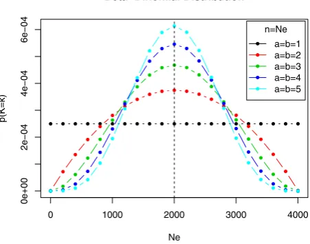
In figure 2, different distributions ofBB(NEktja,b,NE)have been

plotted for different choices ofaandb, whileNE has been chosen

to reflect the size of the functional brain networks. The values given to the parameters (a,b) determine which cost levels are upweighted. In particular, one can observe that EU can be

recovered as a special case ofEBBby selectinga~b~1, as shown

in figure 2. We have here restricted ourselves to symmetric versions of the Beta-binomial distributions, but asymmetric choices are also possible.

Cost-integration over a Subset of the Costs. More generally, cost-integrated metrics can be defined with respect to a subset of the cost regimen. We here illustrate this approach for the case of uniform cost-integration. This perspective on the problem of weighted network comparison has been utilized by several authors [5,7,30]. In our notation, a subset of the cost levels will be indicated by an interval of the form½k{,kz(VK, which

Figure 2. Symmetric versions of the Beta-binomial distribution for different choices of parameters, withNE~4005.

refers to a finite number of values of K, satisfyingk{ƒkƒkz.

Integration over that subset is then defined as

EU(Gjk{,kz):~ X NI kz

t~_{NI k}{

E(c(G,kt))p(ktjk{,kz), ð23Þ

where the probability mass function on K is normalized with respect to the chosen domain of integration ½k{,kz, such that p(kjk{,kz)~1=(NIkz{NIk{z1), for everykin that interval.

The computational formula for this generalization of equation (19) is then given by

EU(Gjk{,kz)~

1

NIkz{NIk{z1 X NI kz

t~_{NI k}{

E(c(G,kt)), ð24Þ

which follows from NIkl~l, using the definition of cost in

equation (7). Note that the value of the conditional probability p(kjk{,kz) will be different if semi-open intervals such as

(k{,kz are considered, instead of closed ones. This is due to the fact that the interval of interest is over a set of discrete values, as opposed to a subset of the real line. As a special case, this notation can also handle the estimation of a particular topological metric at a single cost level, sayk0. In such cases, the interval of

interest becomes½k0,k0. Our notation makes explicit the fact that

integration over a subset of the full cost regimen, is conditional on the choice of such a subset.

Since K has been treated as a random variable and because E(c(G,K))is a function ofK, it follows thatE(c(G,K))is also a random variable. The integralEU(G)can therefore be seen as the

expectation ofE(c(G,K)) with respect to the distribution of K. This probabilistic treatment of cost-integrated metrics will be particularly helpful when considering how to estimate these quantities, as a Monte Carlo (MC) sampling scheme can readily be devised in order to approximate EU(G), when the network of

interest is too large to be computed exactly. More details about this sampling scheme are given in Methods A.

Pros and Cons of Integrating over Cost Levels

We now turn to the main question tackled in this paper: Is it useful to integrate over the different cost levels of a particular weighted network? In order to answer this question, we briefly consider some of the alternatives to this approach. This consists of (i) fixing a cutoff point, (ii) fixing a cost regimen, (iii) integrating over all cost levels, and (iv) directly using weighted topological metrics. Our comparison of these four approaches is substantiated by some simple examples, synthetic data sets, and theoretical results. For convenience, we will solely treat the case of two weighted networks in this section. Extensions of these ideas to the case of several populations of networks are discussed in the Discussion.

Fixing a Cutoff Threshold. The simplest way of comparing the topology of weighted networks is to threshold the corresponding association matrices at a specific value, and evaluate the resulting discrete topologies. It is instructive to study the consequences of such a naive thresholding on two networks with proportional association matrices, as we describe in the following example.

Example 1 Let two weighted networks G1~(V,E,W1) and

G2~(V,E,W2), with standardized association matrices denoted

W1andW2, respectively; such that everywij,k[(0,1)wherek~1,2

labels the two graphs under scrutiny. In addition, assume that

W1:~aW2, ð25Þ

wherea[(0,1)is a scalar. That is, the association matrix ofG2is

simply proportional to that ofG1. Two such association matrices

have been discussed in the introduction and were illustrated in panel (a) of Figure 1. Note that the relationship in equation (25) implies that the diagonal elements ofW1are not standardized to 1:0. However, the topology and cost of weighted networks solely depend on the off-diagonal elements of such association matrices. Therefore, differences in the diagonal elements do not pertain to this discussion. Interestingly, it is easy to show that proportionality in association matrices implies proportionality in weighted cost. Using equation (9), we have

KW(G2)~ 1

NI X

I(G₁₎

awij,1~aKW(G1), ð26Þ

sinceais applied elementwise. Therefore,KW(G2)wKW(G1) as

by assumption0vav1_.

A naive approach to the problem of comparing the topologies of these two networks may proceed by thresholdingW1andW2at a

particular value, say c, as was done in the introduction. If we compare these networks in terms of global efficiency, straightfor-ward computation of the two corresponding quantities shows that we necessarily have

E(k(G2,c))§E(k(G₁,c)), ð27Þ

for any c_{[½0,1, where k(G}

k,c):~I fWkwcg. This follows

sinceG2, thresholded atchas all the edges ofk(G1,c), as well as

additional links owing to its weighted cost being higher. The relationship in equation (27) is then deduced from the monoto-nicity of the efficiency function with respect to cost. Note that these inequalities would hold for both local and global efficiencies, or any other topological metric, which is a monotonic increasing function of the cost level. Therefore, example 1 has shown that thresholding weighted graphs at a fixed cutoff point is misleading, since graphs with higher weighted cost will tend to be classified as having higher levels of global efficiency. This problem can be remedied by fixing cost levels instead of cutoff points.

Fixing a Cost Level. A natural approach to the problem of separating cost from topology is to choose a particular cost level. This may be a single value or a subset of the cost regimen. Such a strategy has been adopted by several authors [5,7,30]. One of the original justifications for conditioning over a subset of the cost regimen was that topological metrics such as CPL or CC cannot be computed for disconnected networks, thereby making it impossible to calculate these quantities for small cost levels. However, since comparable global and local topological properties can also be measured using the efficiency metrics introduced by Latora et al. [19], such problems do not arise when using these topological metrics. We illustrate the consequences of integrating over a subset of the range ofKwith a real data example, where the original data has been transformed. We have constructed a pathological case, which shows that integrating over a subset of the cost levels can fail to distinguish between topologically distinct weighted networks.

Example 2We here consider a single functional connectivity matrix W, corresponding to the mean statistical parametric network (SPN) of a previously published data set [31]. The matrix Wwas transformed in order to produce two other matrices with

Wreg:~Freg(W) andWhyb:~Fhyb(W), respectively. The

func-tionsFregandFhybsimply re-organize the position of the entries in

W, as can be seen from Figure 3. The choice of these transformations was constrained by the following prescriptions,

c Greg,k 0

~c Ghyb,k 0

and c Greg,k 00

~c Ghyb,k 00

, ð28Þ

for cost levelsk0:~0:25 and k00:~0:75, respectively. That is, the adjacency matrices corresponding to costs k0 and k00 are identical forWreg andWhyb. The effect of the functionsFregand

Fhyb was to create different layers of topological structures that

vary according to wiring cost. The hybrid matrix was composed of alternating layers of random and regular topologies. Roughly, the three layers of the hybrid network corresponding to an hybrid association matrix can approximately be described as follows,

topology c(Ghyb,k)

~

Random if k[½0,k0,

Regular if k[(k0,k00,

Random if k[(k00,1:0; 0

B B

@ ð29Þ

for everyk[½0,1, wherekcan only take a finite number of values in the unit interval. The regular matrix, by contrast, was built as three layers of regular topologies. That is,

topologyc(Greg,k)~Regular, ð30Þ

for everyk[½0,1. The random and regular layers were constructed in a standard fashion [31]. Matrices W, Wreg and Whyb

corresponding to weight setsW,WregandWhyb, are represented

in Figure 3 with the corresponding adjacency matrices resulting from different choices of cost levels.

By construction, the weighted graphs Greg~(V,E,Wreg) and

Ghyb~(V,E,Whyb) have identical levels of general efficiency for

the cost levels comprised in the interval ½k0,k00. Therefore, integrating over that interval gives the same result for both graphs:

E

½k0,k00(Greg)~E½k0,k00(Ghyb)¼ :

0:708, ð31Þ

where ¼: means approximately. By contrast, the general efficiencies of these two networks differ substantially when uniformly integrating over the full range of cost, i.e. ½0,1. This gives

EU(Greg)¼: 0:662 and EU(Ghyb)¼: 0:679: ð32Þ

This is as expected, since the hybrid network has several layers of random topologies, which renders it more globally efficient than Greg.

Example 2 illustrates the problems associated with integrating over a subset of the cost regimen. By doing so, we are potentially omitting substantial topological differences between the networks of interest at other cost levels. The difference inEU betweenGreg

andGhyb reported in that counterexample may not appear very

large. However, these two networks could have represented the mean networks of two populations of interest. Providing that the pool of subjects is sufficiently large, such topological differences could be found to be statistically significant. By contrast, comparison of these two networks on the basis of the full cost regimen yielded answers, which were exactly identical, thus nullifying any statistical test of group differences. Naturally, this example could have been constructed in the opposite direction in order to show that networks that seem to differ topologically for some cost subsets are, in fact, identical when uniformly integrating over the full cost regimen.

Fixing a cost level or a subset of the cost regimen therefore suffers from two main problems. Firstly, the arbitrariness of the choice of a specific cost subset will generally be difficult to justify from either a theoretical or a practical perspective. Secondly, as we have illustrated with example 2, considering only a subset of the cost potentially omits topological differences, which are solely visible at other cost levels. Thus, any network analysis using this strategy can only draw conclusions that areconditionalon the choice of cost subset, and this dependence should be made explicit when

Figure 3. Simulation framework for example 2.The small-world correlation matrixWis transformed into a regular and a hybrid matrix, denoted

WregandWhyb, respectively. The regular matrix exhibits a lattice-like topology throughout its cost range, whereasWhyb consists of alternating topological layers of random and regular structures. The entries in both matrices have been arranged in decreasing order from the diagonal, to facilitate visualization.

reporting the results of such analyses. Nonetheless, fixing a particular cost subset successfully satisfies one of our desiderata, which was to disentangle differences in cost from differences in topology. That is, weighted networks’ topologies can be compared irrespective of cost differences, by conditioning on some subset of the cost levels. This invariance property will be made mathemat-ically more precise in the next section.

Integrating over Cost levels. From a statistical perspective, the problem of isolating topology from connectivity strength may be reformulated as evaluating topological differences while ‘controlling’ for cost, where these two quantities are treated as random variables. A natural starting point is to consider weighted networks whose association matrices are proportional to each other, as in the ensuing example.

Example 3 As a simple example, consider the following problem. Let two weighted networks G1~(V,E,W1) and

G2~(V,E,W2), be characterized by the following standardized

association matrices:

W1:~

0:0 w12,1 0:0

, and W2:~

0:0 w12,2 0:0

, ð33Þ

where we assume thatw12,1andw12,2are comprised in the open

interval (0,1). Here, there are only two levels of cost,K[f0,1g. Trivially, G1and G2can therefore be shown to exhibit identical

general efficiency for these two cost levels. Since our proposed formula for cost-integrated topological measures in equation (19) does not include the null cost, we simply haveVK~f1g, which

implies that both graphs attain the maximal level of uniformly cost-integrated efficiency. That is, considering a uniform distribu-tion overK, we have

EU(G1)~EU(G2)~1:0: ð34Þ

This simple example serves as a justification for our exclusion of the null cost from the setVK in equation (16). Including the null

cost would result inEU~0:5for these two basic networks, which

does not appear satisfying. Crucially, the equality in (34) does not depend on the relationship between w12,1 and w12,2. That is,

differences in weighted cost have no impact on cost-integrated topology. We now return to the case studied in example 1 in order to elucidate the exact effect of cost-integration.

Example 1(Continued) In this example, we considered two networks with proportional association matrices, satisfying W1:~aW2. An application of the uniformly cost-integrated

metrics described in equation (19) to the networks of this example gives the following equalities,

EU(W1)~EU(aW2)~EU(W2): ð35Þ

That is, when uniformly integrating with respect to the cost levels, we are evaluating the efficiencies of G1 and G2 at NI discrete

points. At each of these points, the efficiency of the two networks will be identical, becauseW1is proportional toW2and therefore

the same sets of edges will be selected. Thus, G1 and G2 have

identical cost-integrated efficiencies.

The equalities derived in these two examples can be shown to hold in a more general sense. The invariance of cost-integrated efficiency turns out to be true for any monotonic (increasing or decreasing) transformation of the association matrix and applies to any topological metric,T, that takes an unweighted graph as an argument, as formally stated in the following result.

Proposition 1 Let a weighted undirected graphG~(V,E,W). For any monotonic functionh(:)acting elementwise on a real-valued matrix,W, corresponding to the weight setW, and any topological metricT, the cost-integrated version of that metric, denotedTp, satisfies

Tp(W)~Tp(h(W)), ð36Þ

where we have used the association matrix,W, as a proxy notation for graphG.

A proof of this result is provided in Methods B. It relies on the idea that the evaluation of a weighted network solely depends on the ranking of the off-diagonal elements ofW(i.e. the ranking of the elements in W), and that the ranks of a set of values are independent of a monotonic transformation of these values. Note that the arguments used in Methods B do not rely on the definition ofT, nor on the choice ofp(K). Therefore, proposition 1 is true for any cost-integrated topological metrics –i.e. a metric originally defined in a discrete setting for an unweighted graph, and integrated with respect to cost, when applied to a weighted network. Note also that proposition 1 only holds for all levels of sparsity of G if the thresholding function c(G,k) used in the computation of a cost-integrated metric preserves the original ordering of elements inWwith tied ranks, using their indices. In general, however, sparse networks may better be dealt with, in this context, by adjusting the size of the integration domain.

Proposition 1 encapsulates both the advantages and limitations of cost-integrated topological metrics. Two weighted networks, whose topologies are roughly identical at every cost level will be given identical scores under this family of metrics, irrespective of cost differences. Cost-integrated metrics are therefore successful at winnowing topology from connectivity strength. Another singular advantage of this approach is that we obtain a measure, which is invariant under any normalization or standardization of the original data. That is, any functions that simply rescale or shift the association weights, in order to ensure that they are comprised in the unit interval, for instance, will have no effect on the value of the cost-integrated topological measures.

However, proposition 1 also demonstrates the limitation of such an approach. One can easily see that such cost-integration will potentially mask some cost-specific topological differences, as illustrated in example 2. In addition, when cost-integrated topological metrics are used for network comparison, this requires that the sizes of the weight sets of different networks are identical. Similarly, the presence of multiplicities in the ranks of the weights may also cause problems, as this would artificially induce a random topological structure, since weights with equal ranks would be randomly allocated to different cost levels. We will further discuss these limitations in the conclusion of this paper.

Using a Weighted Metric. A seemingly natural way of amalgamating connectivity strength and topological characteristics is by directly considering weighted topological metrics, such as the weighted global efficiency, EW, introduced in equation (14).

Unfortunately, we here prove that such an approach suffers from a serious limitation, which could potentially dissuade researchers from using this particular type of metrics. With the next proposition, we show that in a wide range of settings, the weighted efficiency is simply equivalent to the weighted cost of the graph of interest.

Proposition 2For any weighted graphG~(V,E,W), whose weight set is denoted byW(G), if we have

min wij[W(G)wij

§1

then

EW(G)~KW(G): ð38Þ

This result can be proved by contradiction, as demonstrated in Methods C. The hypothesis in proposition 2 may at first appear relatively stringent. However, it will encompass a wide range of experimental situations. For the real data set described in example 2, the difference betweenmaxwijand2 minwijis close to, but not

exactly, zero. However, we nonetheless haveEW~KW, for that

example. Thus, the added value of using the weighted efficiency will, in general, be questionable since there exists a strong relationship between this topological measure and a simple average of the edge weights.

These theoretical results and associated counterexamples have therefore highlighted the limitations of various approaches to the problem of disentangling differences in cost from differences in topology. As a result, when comparing several populations of networks, we recommend the reporting of differences in weighted costs and differences in cost-integrated topological measures. We illustrate this approach with a re-analysis of a previously published fMRI data set.

N-back Working Memory Data Set

In this section, we illustrate our theoretical results with a previously analyzed data set of a working memory task based on functional Magnetic Resonance Imaging (fMRI) data [31]. In particular, we use this data set for testing our proposed MC sampling procedure and for comparing a graph’s weighted cost with its cost-integrated and weighted global efficiencies.

Description. Ginestet et al. [31] considered topological changes in functional brain networks under different levels of cognitive load. Here, we give a cursory description of the experimental procedure used in this study and refer the reader to the original paper for the full technical details. Ginestet et al. [31] constructed networks on the basis of fMRI data gathered from 43 healthy adults undergoing a working memory task known as the N-back paradigm. Echo planar imaging data quality was assessed using an automated technique [32]. In this experiment, subjects were shown one letter every two seconds, and were asked to monitor the stimuli, in order to indicate by the push of a button whether the current letter was identical to the one presentedN trials previously, whereN~_f1,2,3g. A control or null condition was also included, the 0-back task, which consisted of simply indicating whether the current letter was an X. In this experiment, the subject-specific fMRI images were parcellated into 90 regions of interest using the Anatomical Automatic Labelling (AAL) template [33]. The BOLD time series were averaged for each AAL region. These regional mean time series were then wavelet decomposed. Wavelet coefficients in the low frequency range (0.01–0.03 Hz) were selected for the main network analysis [6]. Since theN-back paradigm contains four experimental levels, we decomposed these time series into blocks corresponding to each N-back condition. As each condition was repeated more than once, these blocks were then concatenated. Note that this sequence of processing steps involving wavelet decomposition immediately followed by block concatenation was studied by Ginestet et al. [31] using simulated data, and was not found to bias the results of the final network analysis.

Vertices in these subject-specific functional networks were chosen to be the 90 AAL regions, and the edges were constructed by computing pairwise correlations between each condition-specific time series of wavelet coefficients. The results of this

construction can be summarized using Statistical Parametric Networks (SPNs), as illustrated in Figure 4 [31]. SPNs are estimated using a mass-univariate approach, where the edges in a population of subject-specific networks are tested for significance using a mixed-effects model, and then thresholded using the false discovery rate [34,35]. SPNs can be constructed using functions made freely available through the R package NetworkAnalysis (http://CRAN.R-project.org/package = NetworkAnalysis). From Figure 4, one can observe that the connectivity strength (i.e. weighted cost or averaged correlation coefficient) of the functional networks in each condition tend to diminish as subjects experience greater cognitive load.

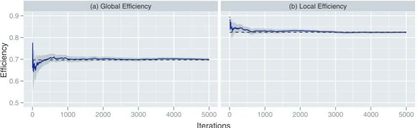
Monte Carlo (MC) Estimation. A full description of the theory supporting MC estimation in this context is provided in Methods A. MC techniques are here used to speed up the computation required when estimating our proposed cost-integrated measures. Figure 5 shows the convergence ofE(m)_U to EU, for a medium-sized weighted network derived from fMRI

data on the working memory task described in example 2. The results are provided for both global and local efficiencies. Each plot in Figure 5 shows the running mean plus or minus twice the running MC standard error, which are defined for the uniformly cost-integrated global efficiency, asE(m)_U and(v(m)_U )1=2, respectively, wherem~1,. . .,5000. (See Methods A for details.) In Figure 5, we also report the exact values ofEU using formula (19) by dashed

lines.

In all the cases studied, the MC estimates compared favorably with the exact integrals after approximately a quarter of the number of computations required for the exact calculations. That is, the exact derivation ofEU necessitatesNI~4005evaluations of

the global or local efficiency. By contrast, MC estimates based on approximately1000samples appear to provide reasonably good approximations of these quantities, as indicated by the small MC standard error. This constitutes a non-negligible computational gain. The MC standard error, which is derived as a by-product of these computations could then be used as an indicator of the uncertainty associated with these estimates in a Bayesian hierarchical model, where uncertainty is propagated from the data to the population’s parameters of interest.

A simple alternative to MC averaging, in our context, would be to construct a mesh of the unit interval and to approximate the desired integral by a weighted sum of the values of the topological metric of interest at the midpoints of that mesh. The latter method is generally referred to as the Gauss-Kronrod quadrature formula [36]. While this method is very efficient for simple functions, it becomes rapidly unwieldy for complex ones, as it requires an increasingly refined mesh to ensure good interpolation. Moreover, since the Gauss-Kronrod is a deterministic algorithm, it does not provide a measure of the accuracy of the estimation. By contrast, a MC approach ensures asymptotic convergence for any level of complexity and also produces precise confidence bands. (See Methods A for details.)

Evaluation and Comparison. Following the statistical framework used in the original analysis of this data set [31], we tested for the statistical significance of the N-back factor on different topological metrics using a mixed-effects model. We here haven~43subjects andJ~4experimental conditions. Using the formalism introduced by Laird et al. [37], we have

y_i ~XibzZibiz[i, i~1,. . .,n,

[i* iid

N(0,s2

[I) bi* iid

N(0,s2 bI),

ð39Þ

topological metrics of interest, b:~½b₁,. . .,b_JT is a vector of fixed effect, which do not vary over subjects,bi:~bi1is a

subject-specific random effect and ei:~½[i1,. . .,eiJT are the residuals.

Finally, the matrices Xi’s and Zi’s are given the following

specification,

Xi~

1 0 0 0

1 1 0 0 1 0 1 0 1 0 0 1 2

6 6 6 4

3 7 7 7

5, and Zi~

1

1 1 1 2 6 6 6 4

3 7 7 7

5, ð40Þ

for every i~1,. . .,n. The effect of the N-back factor was then evaluated using Wald’sF-test. All these analyses were conducted within the R environment using the lme4 package [38]. Note that the model used here is slightly simpler than the one used in Ginestet et al. [31], as the present mixed-effect model was found to be better identified than the growth curve model utilized in the original analysis.

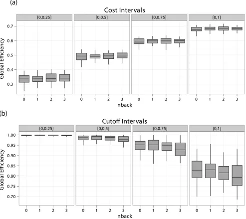
In Figure 6, we report the cost–integrated global efficiencies for this experiment. For illustrative purposes, we have computed these quantities for four different choices of domains of integration. The EGlo

U (Gijjk{,kz) were here estimated using

1,000 MC samples for each subject in eachN-back condition. In panel (a), one can observe a clear increase of the cost-integrated global efficiencies as we increase the size of the domain of integration, due to the monotonicity of global efficiency with respect to cost. This is a standard property of global efficiency: as graphs become denser, their diameter tends to diminish [39]. In Figure 6, one can also note the dependence of the inter-subject variability of the cost–integrated metrics on the chosen domain of integration.

We therefore tested for the effect of theN-back factor on the topological metrics of interest, given different domains of integration, in order to evaluate whether such a choice of domain has a systematic impact on the effect of the experimental factor. These tests are based on the mixed-effects model described in equation (39), and we have reported the results of these statistical tests in Table 1. These results do not indicate that the choice of different domains of integration or the choice of different specifications of the Beta-binomial distribution yield systematic biases in statistical inference. As was reported by Ginestet et al. [31], the weighted cost was found to be systematically affected by the N-back factor (WaldF~3:59,df1~3,df2~126,p~0:01).

However, none of the cost-integrated global efficiencies appeared to be significantly influenced by the experimental factor. Most

Figure 4. Mean Statistical Parametric Networks (SPNj) over the 4 levels of theN-back task, in the sagittal plane, based on wavelet

coefficients in the 0.01–0.03 Hz frequency band, with FDR correction (base ratea0~:05).Locations of the nodes correspond to the stereotaxic centroids of the corresponding cortical regions. The inferior–superior orientation axis is indicated in italics. The size of each node is proportional to its degree.

doi:10.1371/journal.pone.0021570.g004

Figure 5. Running means of Monte Carlo (MC) estimates for uniformly cost-integrated global and local efficiencies in panels (a) and (b), respectively, for the3-back network described in example 2.The grey ribbon represents the variability of these estimators at each

m~1,. . .,5000, using twice the MC standard error. That is,E_U(m)+2s(_Um)for both global and local efficiencies. The dashed lines indicate the exact value

ofEU. See Methods A for details.

importantly, neither the use of different domains of integration nor the specification of different parameters for the Beta-binomial distribution seemed to affect the results. Integration over the entire cost domain, however, resulted in a largerF-statistic, which may be explained by the lower amount of variability characterizing cost-integration over larger cost domains, as can be observed in Figure 6. In panel (b), cost-integrated efficiencies with respect to the Beta-binomial distribution for several choices of parameters indicate that a possible relationship between global efficiency and cognitive load may exist. However, this relationship did not reach statistical significance, as can be seen from Table 1. It therefore appears that although different choices of probability mass functions onKyielded slightly different results, the overall analysis

seems to indicate that the experimental factor was not a predictor of global efficiency.

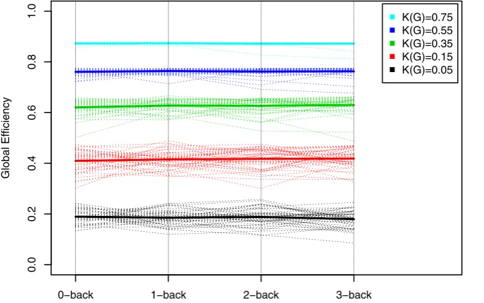
In addition, in Table 1, we have also reported theF-statistic for the effect of theN-back factor on the weighted cost. The subject-specific network’s weighted costs were found to be significantly influenced by the level of the experimental factor, as is immediately visible from the mean SPNs reported in Figure 4. The separation of the differences in cost from the differences in topology that results from the use of a cost-integrated topological metric is best illustrated by the interaction plots in Figure 7, where ensembles of global efficiencies corresponding to different costs are represented for the four levels of the experimental factors. Note that, here, we are reporting the efficiency metrics for a single level

Figure 6. Box plots of cost-integrated global efficiencies. In panel (a), uniformly integrated and in panel (b), Beta-binomial cost-integrated global efficiencies of fMRIN-back networks for four different domains of integration and different choices of parameters are represented. These integrals were estimated using MC approximation over 1,000 samples for each of the 43 subjects in each of the four experimental conditions. Note that different domains of cost-integration do not induce any differences in the effect of the experimental factor, in panel (a). However, the use of the Beta-binomial distribution seems to indicate that a gradual increase in global efficiency follows an increase in cognitive load, in panel (b). However, these relationships did not reach statistical significance (see Table 1).

of cost, not integrated over a subset of the cost regimen as was done in Figure 6. This is a visual depiction of theN-back factor that corroborates the conclusions reached using cost-integrated topological metrics, which stated that topology, as measured by global efficiency, does not significantly vary with the experimental factor.

Discussion

This paper has investigated the effect of thresholding matrices of correlation coefficients or other measures of association for the purpose of producing simple unweighted graphs. On the basis of this analysis, and the examples studied in this paper, we make the following methodological recommendations to researchers intend-ing to compare the topological properties of two or more populations of weighted networks.

Summary and Recommendations

We here summarize the main findings of this paper: (i) fixing a cutoff threshold is not satisfactory, because this is fully determined by differences in connectivity strength, as we have shown previously; (ii.) fixing a subset of cost levels is not satisfactory, because this potentially omits topological differences at other cost levels; (iii) integrating over the entire cost regimen successfully disentangles connectivity strength from topology up to monotonic transformations. Specifically, such metrics are invariant to monotonic transformations of the association weights; and (iv.) the weighted topological metrics, such asEW, appear to be too

closely related to weighted costs.

From a methodological perspective, we therefore recommend the following. As a preliminary step, it is good practice to standardize the association weights, in order to obtainwij[½0,1for

allwij’s, with large values of the weights corresponding to strong

associations, although some care must be taken in the interpre-tation of the resulting standardized weights. This may facilitate comparison across separate network analyses, and ease the interpretation of the results. Secondly, the weighted cost, i.e. connectivity strength, of the networks of interest can then be computed for all networks. This is central to the rest of the analysis, and should be conducted systematically. Moreover, quantitative differences in connectivity strength per se are informative about the brain processes at hand, and their experimental relevance should not be neglected. Thirdly,

Table 1.Statistical inference for the mixed-effects model described in equation (39).

Outcome Variable Cost Domain F-statistic p-value

KW(G)

Weighted Cost 3.59 0.01

EGlo

U (Gjk{,kz)

Cost-integrated ½0,:25 0.34 0.79 Cost-integrated ½0,:50 0.24 0.86 Cost-integrated ½0,:75 0.40 0.75 Cost-integrated ½0,1:0 1.09 0.35

EGlo

BB(Gja,b)

Beta-binomial,

a~b~1

½0,1:0 1.09 0.35

Beta-binomial,

a~b~2

½0,1:0 0.94 0.42

Beta-binomial,

a~b~3

½0,1:0 0.97 0.41

Beta-binomial,

a~b~4

½0,1:0 1.37 0.25

Testing of the effect of theN-back factor on global efficiency. For uniformly cost-integrated (EU) global efficiencies, we have separately tested four different

domains of integration, whereas for Beta-binomial (EBB) cost-integration, we

have considered four different specifications of the parameters of the Beta-binomial distribution.

doi:10.1371/journal.pone.0021570.t001

Figure 7. Interaction plots of cost-dependent global efficiencies of fMRI networks with respect to the levels of theN-back factor.We here consider five different costsK[f0:05,0:15,0:35,0:55,0:75g. The dashed lines represents the cost-specific global efficiencies for each subject, whereas the plain line represents cost-specific global efficiencies averaged over the 43 subjects. The flatness of the lines at each cost levels suggests that the experimental factor has little effect on the topological structure of these networks.