Do simplifications in the intitial set up matter?

Do simplifications in the initial set-up matter?

Lucas C.A. Braam

Department Aerospace Engineering

San Diego State University

San Diego, CA 92182-1308

Email: [email protected]

Gustaaf B. Jacobs

Department of Aerospace Engineering

San Diego State University

San Diego, CA 92182-1308

Email: [email protected]

Corresponding author

Kees H. Venner

Department of Eng. Fluid Dynamics

Universiteit Twente

Enschede, The Netherlands, 7500 AE

Email: [email protected]

August 1, 2018

1

Abstract

The Richtmeyer-Meshkov instability occurs in a number of flow application. Therefore, some experimental and numerical studies have been conducted. But during the numerical studies some simplifications are made to reduce computational time. In this paper, there is investigated what the effects are of these simplifications on the particle cloud. This will be done with two-dimensional simulations of a shockwave hitting particle cloud with a volume fraction lower than 3 %. The simulations focus on the effect of particle response time, a Gaussian distributed particle diameter, a random uniform distributed initial particle cloud and particle collisions. Al these phenomena have an effect to a varying degree on the number density distrubution, the x-location and width of the cloud

2

Introduction

The first theory describing the instability on the interface of two fluids with different densities caused by the acceleration of one fluid into the other fluid, was developed by G.I Taylor. His theory describes the growth of the irregularities on the interface of the two fluids, which later became known as the Rayleigh-Taylor instability (RTI)[1].

This instability occurs in many flow applications, from high speed combustion too dust explosions. In these examples a special type of RTI occurs, namely: The Richtmeyer-Meshkov Instability (RMI). A shockwave ini-tiates the RMI, so the acceleration is no longer constant, and can be seen as an impulsive acceleration. This impulsive acceleration amplifies the initial perturbation on the interface. Richtmeyer[2] was the first to describe this problem. His theories were later confirmed by Meshkov[3].

The RMI is a result of misalignments of the local density gradients and the pressure gradients on the interface. These misalignments generate baroclinic vorticities. These baroclinic vorticities amplify the initial perturba-tions. This growth of the pertubations enters the nonlinear regime, with blobs of the light density fluid moving into the heavy density fluid and blobs of the heavy density fluid moving into the light density fluid. [4]. The majority of the studies of RMI focus of on the interface between two fluids with different densities. Far less studied is the problem of a curtain of particles, which is accelerated by a shock wave. Some studies dedicated to dispersed phase flows, flows with a dispersed phase of particles, have been conducted. For instance by Boikoel al [5], who studied the interface between a shock wave and a cloud of particles experimentally and numerically. Further numerical studies of this problem have been conducted by Jacobsel al [6]. In these numerical studies the initial particle cloud was simulated as an uniform distributed curtain of particles, with constant diameter. Furthermore, there are no mentions of a particle collision model in these papers. These simplifications could cause for differences between the numerical results and reality

curtain of particles. This is done by varying the particle distribution as well as the diameter of the particles. In later the stages of this paper, a simple particle collision model will be introduced, to study the effect of particle collisions.

In the first section the governing equations and the physical model will be given. Next, the numerical model will be explained. Finally, the initial set-up and the results will be evaluated, followed by the conclusion.

3

Governing equations

The problem is modelled with the particle-source-in-cell (PSIC) method [7]. This method tracks the particles in a Lagrangian frame and solves the the conservation equations for the carrier flow in the Eulerian frame. In the rest of the paper, variables with the subscribedpwill be particle variables and variables without a subscript will be fluid variables unless stated otherwise.

3.1

Gas Phase

As mentioned, the conservation equations form the governing equations of the carrier flow. These equations are given in dimensional form in the next subsection and later the method for rewriting the equations into non-dimensional form is given.

3.1.1 Dimensional form

The two-dimensional Euler equations in Cartesian coordinates are given below. A source term is added to these equations to ensure two-way coupling between the carrier flow and the particles.

Qt+Fx+Gy =S, (1)

where

Q= (ρ, ρu, ρv, E)T, (2)

F = (ρu, ρu2+P, ρuv,(E+P)u)T, (3)

G= (ρv, ρuv, ρu2+P,(E+P)v)T (4)

and

P= (γ−1)E−1

2ρ(u

2_+v2_{), γ= 1.4. (5)}

This system of equations is closed with the equation of state:

T =γP M

2

ρ , (6)

where the reference Mach number is given byMref =Uref/

p

(γRTref). In the simulations the reference Mach

number is set to be unity [6].

3.1.2 Non-Dimensional system of equations

The governing equations shown in the previous paragraph are rewritten in non-dimensional form to reduce the number of free parameters and thus, to simplify the analysis.

Four reference values are used to obtain the non-dimensional form. These being Uref, ρref, Lref and Tref.

Using these reference values gives nine non-dimensional variables, all non-dimensional variables in the paper are denoted with a bar on top, except in figures, where all variables are non-dimensional, unless stated otherwise.

¯

u=u/Uref, (7)

¯

v=v/Uref, (8)

¯

ρ=ρ/ρref, (9)

¯

x=x/Lref, (10)

¯

y=y/Lref, (11)

¯

T =T /Tref, (12)

¯

P =P/(ρrefUref2 ), (13)

¯

E =E/(ρrefUref2 ), (14)

¯

Furthermore, there are two more variables that are used to describe this problem, namely, the Reynolds number and the particle response time, which is an indicator for the time a particle needs to react to changes in the carrier flow. Their formula’s are given in equations 16 and 17, respectively.

Re= ρrefLrefUref

µ , (16)

τp=

ρpd2p

18µ [t], (17)

whereµis the dynamic viscosity after the shock.

The particle response time will be rewritten in a non-dimensional form.

¯

τp=

τpUref

Lref

=ρpd

2

pUref

18µLref

Reµ ρrefLrefUref

= Reρpd

2

p

18ρrefL2_ref

=Reρ¯p ¯

dp

2

18 .

3.2

Dispersed Phase

Kinematic equations are used to track the motion of the particles, this is done in a Lagrangian frame. Below the equation for the particle’s position~xp is given.

d~xp

dt =~vp, (18)

where~vp is the velocity vector.

The particles are accelerated by the drag force on the particles, this is in accordance with Newton’s second law. Furthermore, the particles are assumed to be spherical and the drag is taken as a combination of pressure drag and Stokes drag with corrections for high Reynolds and Mach numbers. This leads to the following equation governing the particle velocity[6]

~vp

dt =f1

~v_f−~v_p τp

− 1

ρp

∇P|f (19)

In this equation,~vf is the velocity of the fluid at the particle position. The first term on the right hand side

of the equation describes the contribution of velocity difference between the particle and the carrier flow to the particle acceleration. f1 in this term is an empirical correction factor [5], which gives results within a 10% of

measured particle acceleration for higher relative particle Reynolds numbers up toRef = 10,000 and relative

particle Mach number up toMf =|~vf|/pTf = 1.2

f1=

3

4(24 + 0.38Ref + 4

p Ref)

1 +exph−0.43 M4.67

f

i

(20)

The second term describes the particle acceleration caused by the pressure gradient in the carrier flow at the particle position.

The equation for temperature is given as,

dTp dt = 1 3 N u P r

T_f−T_p τp

. (21)

This equation is derived from the first law of thermodynamics and Fourier’s law for heat transfer. In this equation the Prandtl number set to beP r= 1.4, andN u= 2 +p

RefP r0.33 is the Nusselt number corrected

for high Reynolds number[6].

3.3

Source term

The momentum and energy generated by the particles affects the carrier flow. The volume averaged contribu-tions are summed in the a continuum source term, which gives a contribution to the the momentum and energy equation in 1 as:

~ Sm(~x) =

Np X

i=1

~ Se(~x) =

Np X

i=1

K(~xp, ~x)(W~m·~vp+We), (23)

where K(x, y) = K(|x−y|)/V is a normalized weighting function that distributes the influence of each particle onto the carrier flow. The weight functions describing the momentum and energy contribution of a particle areW~m=mpf1(v~f−~vp)/τpandW~e=mp(N u/(3P r))(T−Tp)/τp, wheremp is the mass of a spherical

particle, andNp is the total number of particles.

In the code, the source term is computed using the computer particlesNc. To correct this the source is multiplied

by a factor, namely: the source factor. The source factor is a factor between the real number of particles and the number in the computer simulation. The formula for the factor is given below.

Fsource=

Np

Nc

, (24)

4

Numerical model

4.1

WENO-Z

The numerical scheme that will be used too solve the problem is a WENO (Weighted Essentially Non-Oscillatory) scheme. WENO schemes are based on the ENO (Essentially Non-Oscillatory) schemes. This type of scheme was first introduced by Liuet al[8]. These schemes were analysed and improved further along the years[9]. The scheme that will be used to analyse the problem was developed by Jacobset al and is described in [6].

4.2

Gaussian Distributed Diameter

In order to obtain an Gaussian distribution, the Box Muller method [10] is used. This method transforms two uniform random values into a Gaussian random value, using the following equation:

¯

dp=

p

−2log(r)cos(2πs)σ+µr, (25)

whererandsare uniform random variables,σis the standard derivative andµr is the mean diameter.

4.3

Collision Model

The Collision model is modification of a collision model made in Iowa University. The collision model uses Newton’s second law to model the collisions, there is assumed that the two particles have the same mass. The model will simulated a collision when the distance between the two particles is smaller than the critical diameter. The definition for the critical diameter is given in equation 26.

¯

dcric= 1.2·d¯p·Fsource·F2D, (26)

whereF2D is a factor to account for switching from 3D to 2D to model the collisions. This factor are given in

equation 27.

F2D=

2 3 ¯

dp. (27)

To reduce computational time, only the distance between particles that are positioned in the same grid cell is checked. The grid cell location of the particle (Cell) is computed using the following formula:

Cx=IN T

x_p−x₀ Lx(N5−N0)

+N0, (28)

Cy=IN T

y_p−y₀ Ly(M5−M0)

+M0, (29)

Cell= (Cx−N0 + 1)(Cy−M0) +Cy. (30)

In these equationsN0 andM0 are the first grid points in, respectively x and y-directions. N5 andM5 are the final grid points in these directions. Finally, ¯Lx and ¯Ly indicate the length of the domain in both directions.

Errors occur whenCell is equal to zero, too prevented this from happening one is added to the first term on the right hand-side of equation 30.

equation 32. After the transformation, the normal velocities after the collision are computed using the following formula:

unew=

un1+un2

2 . (31)

R=

cos(θ) sin(θ)

−sin(θ) cos(θ)

(32)

un

ut

=R

up

vP

. (33)

Afterunis replaced byunew, the velocities are transformed back to the original coordinate system. The rotation

matrix used for this transformation is shown below.

R=

cos(θ) −sin(θ)

sin(θ) cos(θ)

, (34)

this matrix is filled in equation 33 to obtained the transformation. After theun of the particles is adjusted, the

velocities are transformed back to the original coordinated system with the next rotation matrix,

(a) Free body diagram of the particle collision in orig-inal coordinated system

(b) Free body diagram of the particle collision after coordinated transformation

Figure 1: Free body diagrams of the particle collision

5

Simulation setup

A two-dimensional problem of a moving shock hitting a cloud of particles will be simulated. This two-dimensional problem was studied experimentally by Boikoet al [5].

In the simulation, the ¯τp will be varied in order to analysed the effects of the particle response time on the

results. Furthermore, the influence of the particle distribution in the initial cloud will be analysed. This is done by studying two different cases, namely: an uniform distributed case and a random distributed case.

In these simulations the Reynolds number, given in equation 16, will be 5.152×105_{. The dynamic viscosity (µ)}

used in the calculation is the dynamic viscosity of dry air at temperature of 750K, (µ= 3.482×10−5_kg/ms

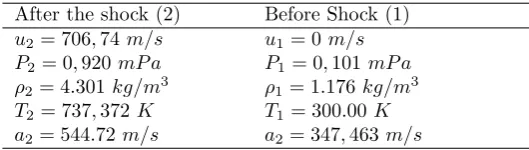
[11]). The rest of the dimensional, non-dimensional and the reference variables are given in the tables below. The relation between these variables is described in subsection 3.1.2. The dimensional values are given in table 2 correspond to a shock with Mach number 2.8 in a shock tube [12].

Table 1: Reference variables

Lref = 0.052m

Uref = 293,41m/s

Tref = 214.88K

ρref = 1.176 kg/m3

Table 2: Problem variables

After the shock (2) Before Shock (1)

u2= 706,74m/s u1= 0m/s P2= 0,920 mP a P1= 0,101 mP a ρ2= 4.301kg/m3 ρ1= 1.176kg/m3 T2= 737,372 K T1= 300.00K a2= 544.72m/s a2= 347,463 m/s

Table 3: Non-Dimensional variables

After the shock (2) Before Shock (1) ¯

u2= 2.4087 u¯1= 0

¯

P2= 8.98 P¯1= 1

¯

T2= 3.421 T¯1= 1.4

¯

ρ2= 3.6636 ρ¯1= 1

As mentioned the ¯τpwill be varied, the particle diameter and the volume fraction will also change accordingly.

The volume fraction of the cloud is calculated by dividing the volume of the particle cloud by the total volume of the particles, the formula is given as:

Fvol=

4 3

Npπ

¯

dp

2

3

hcwc

= 4 3

NcFsourceπ

¯

dp

2

3

hcwc

. (35)

6

Results

The results will be split into 4 subsection. In the first subsection, the effect of ¯τp is discussed. The second

part focuses on an uniform random distributed particle cloud versus a uniform distributed particle cloud. In the third subsection the diameter of the particles will be varied with an Gaussian distribution, and finally, the effect of particle collisions will be investigated.

6.1

Particle response time

In subsection three cases are analysed and compared, the particle response time and the volume fraction for these cases are shown in table 4. All initial particle distribution is uniform random. The average ¯xlocation of the particle is plotted against the non-dimension time in figure 2.

Table 4: Cases

τp Volume fraction

972 3%

729 1.95%

Figure 2: ¯xlocation of the cloud for different particle response times.

As can be seen in the figure, when the particle response time is lower, the particles reacts faster to changes in the carrier flow and thus, the particle cloud moves quicker. This is according to the flowing formula:

dup

dt =

1

τp

|uf−up| (36)

6.2

Uniform Random distribution

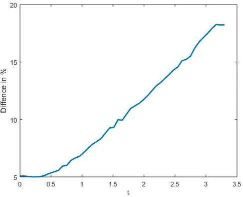
To see the effect of the initial distribution of the particles in the particle cloud, the difference in number density will be plotted. The number density describes the concentration of the particles. The difference in number density is plotted in figure 3. The difference in number density is calculated using this formula:

Dif fφ=

PNx

i=0 PNy

j=0|φai,j−φbi,j|

Nx·Ny

/ PNx

i=0 PNy

j=0φai,j

Nx·Ny

,

(37)

where the superscriptastands for a uniform grid andbfor a random grid.

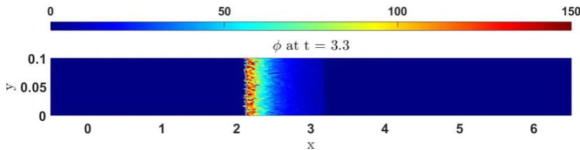
A difference in number density means that the particles are distributed differently in the cloud. In the figure, there can be observed that there already is a difference in number density. The different particle position in the initial cloud causes this difference in number density. This initial difference grows over time. Meaning that the particles concentrated in other positions of the cloud, this is shown perfectly in figures 4 and 5. The distribution of the number density for the random initialized cloud has more fluctuations, especially in the ¯

y-direction. These fluctuations can have huge impacts on the flow-field upstream.

Figure 4: Number density at ¯t= 3.3 of the uniform distributed initial cloud

Figure 5: Number density at ¯t= 3.3 of the random distributed initial cloud

6.3

Gaussian distributed diameter

The effect of the Gaussian distributed particle diameter is studied using three cases, namely, a case with a constant diameter, a case with a standard standard deviation of 5 % of the distribution of the particle diameter and a case with a standard deviation of 10 % of the distribution of the particle diameter.

In figure 6, the variance of the ¯x-location of the particles is plotted. The variance of the cloud gets bigger with an increasing standard deviation. This is due to the wider range of ¯dp, and this leads to a wider range ¯τp

following equation 17. In figure 2, it can be seen that particles with an higher ¯τp react slower to changes in the

Figure 6: Variance of the ¯x-location of the particles plotted against the ¯t

6.4

Particle collision

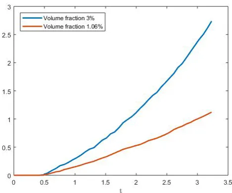
In figure 7, the difference between the results of a code with the random grid and the uniform grid are shown, the formula for the difference is shown in equation 37, where this time the superscriptastands for the uniform grid and the superscriptbdenotes the random grid.

The difference become bigger over time, and the particle collision model has a bigger impact when the volume fraction is higher. Due to the higher number of particles there are more collision, and it has thus a bigger effect on the number density.

Figure 7: Difference in number density caused by the particle collision

Figure 8: Energy loss due to particle collision in percentages

7

Conclusion

To conclude, the simplification in the initial set-up matters to a varying degree. The simplifications can affect the width and position of the particle cloud, also the number density of the cloud is affected by the simplifications. The width of the cloud is mostly affected by the assumption of a constant diameter for all particles. The mechanism behind this phenomenon is the quicker reaction of particles with a smaller diameter to changes in the carrier flow than their larger counterparts. This is caused by the relation between the diameter and the particle response time, smaller particles have a smaller particle response time. This difference in particle response time increases the overall width of the particle cloud.

The location of the particle cloud was mostly affected by changes in the particle response time. This relation is described in formula 36.

The number density of the cloud was affected by some simplifications. The simplification with the greatest effect on the number density is the distribution of the particles in the initial particle cloud. The effect minor in the beginning, but increase over time and in the end could cause a difference of 17% in the end. The effect of particle collisions on the number density was less dramatic for clouds with a low volume fraction. But the effect of the collisions increases, when the volume fraction of the cloud increases.

Finally, there was seen that the effect of particle collision on the total kinetic energy of the particle cloud was negligible for clouds with a low volume fraction.

All these simplifications could cause major differences between the results from the CFD analysis and reality, therefore the effect of the simplifications should always be considered before making them. For this reason, more research should be dedicated to the effects of the simplifications on the carrier flow: How is the pressure of the flow affected?, How is the temperature of the flow affected?, etc.

A

Appendix

This paper is part of a research conducted by the Aerospace Engineering department of the San Diego State University (SDSU). SDSU is a public research university located in the San Diego county, and is the largest and oldest higher education institute of the San Diego county. The research is lead by professor G. Jacobs and focusses on Computational Fluid Dynamics applications.

As described in the paper, mine research focusses on the initial particle cloud and other simplifications. During the research the code created by G. Jacobset al[6] was used to analyse the effects of the initial particle cloud on the final solution. In order create a different initial particle cloud, some subroutines were added to the original code. Later a particle collision model was created and added to the code.

References

[1] J. Taylor, The instability of liquid surfaces when accelerated in a direction perpendicular to their planes, Proc. Roy Soc., J. Loud. ser. A, vol. 201, no. 1065, 1950.

[2] R. D. Richtmyer,Taylor instability in shock acceleration of compressible fluids, Communs. Pure and Appl. Math., vol. la, pp. 297-319, 1960.

[3] E.E. Meshkov, Instability of shock-accelerated interface between two media, Advances in Compressible Tur-bulent Mixing, 8810234:473, 1992.

[4] R.G. Izard, S.R. Lingampally, P. Wayne, G.B. Jacobs, P. Vorobieff,Instabilities in a shock interaction with a pertubecd curtain of particles, Int. J. Comp. Meth. and Exp. Meas., Vol. 6, No. 1 (2018) 5970

[5] V.M. Boiko, V.P. Kiselev, S.P. Kiselev, A.N Poplavsky, V.M. Fomin,Shock wave interaction with a cloud of particles, Combustion, Explosion, and Shock Waves, Vol. 32, No. 2, (1996), DOI: 10.1007/BF02097090

[6] G.B. Jacobs, Wai-Sun Don,A high-order WENO-Z finite difference based particle-source-in-cell method for computation of particle-laden flows with shocks, J. Comput. Phys. 228 (2009) 13651379

[7] M.P. Sharma, D.E. Stock, The particle-source-in-cell (PSI-CELL) model for gas-droplet flows, Journal of Fluids Engineering, Vol. 99, No. 2, (1997)

[8] X-D. Liu, S. Osher and T. Chan,Weighted essentially non-oscillatory schemes, J. Comput. Phys. ll5 (1994) 200-212.

[9] C.W. Shu, S. Osher, Efficient implementation of essentially non-oscillatory shock-capturing schemes, J. Comp. Phys. 77 (1988) 439-471.

[10] G. E. P. Box and Mervin E. Muller, A Note on the Generation of Random Normal Deviates, The Annals of Mathematical Statistics (1958), Vol. 29, No. 2 pp. 610611 doi:10.1214/aoms/1177706645, JSTOR 2237361

[11] Engineering ToolBox, (2005). Dry Air Properties. [online] Available at: https://www.engineeringtoolbox.com/dry-air-properties-d 973.html [23-04-2018]