VIRTUAL SURGERY: Development of a surgical simulation tool for the prediction of functional impairment after partial glossectomy

(1)

VIRTUAL SURGERY

Development of a surgical simulation tool for the prediction of

functional impairment after partial glossectomy

(2)

(3)

Kilian D.R. Kappert

Technical Medicine – Medical Imaging and Intervention September 2015 – August 2016

Masters Graduation Committee

Chairman and external member Prof T. Ruers, MD, PhD

Department of surgical oncology

Netherlands Cancer Institute, Amsterdam, The Netherlands

MIRA institute for Biomechanical Engineering and Technical Medicine University of Twente, Enschede, The Netherlands

Clinical supervisor Prof A.J.M. Balm, MD, PhD, FACS, FRCS

Department of Head and Neck Oncology and Surgery Netherlands Cancer Institute, Amsterdam, The Netherlands

Technical Supervisor F. van der Heijden, PhD

Mentor P.A. van Katwijk, Msc.

Additional member M.J.A. van Alphen, PhD

Department of Head and Neck Oncology and Surgery Netherlands Cancer Institute, Amsterdam, The Netherlands

VIRTUAL SURGERY

(4)

Preface

(5)

Summary

Introduction: Prediction of functional consequences of a partial glossectomy can be difficult because of the complex synergistic activities of many muscles and neural structures involved in the swallowing and speech process. Predicting these functional consequences could give both the surgeon and the patient the information they need to choose the right treatment.

Method: In this report a tool to perform surgery on a finite element based biomechanical model of the tongue is presented. The tool enables removal of a volume from the model and suturing of the virtual wound. In addition, scar tissue is added. The biomechanical model itself is an edited version of an existing biomechanical model. To make editing of the biomechanical model possible, the finite element and surface mesh are separated. The surgery tool is validated using real patient cases. From these patient cases, pre and postoperative 3D videos are analysed and compared with the biomechanical tongue, edited by the surgical tool.

Results: The new biomechanical tongue model is comparable with the model on which it is based. Only the Superior longitudinal- and Hyoglossus muscle have different volumes and act slightly different. Patient cases show that the biomechanical model is able to give a qualitative indication about the direction of impairment after surgery. Quantitative comparison is not yet possible because of the restrictions of the measurement method to measure the movement of the patient’s tongue.

Conclusion: In this report the next step towards prediction of functional outcome of a glossectomy is made. After personalising the tongue shape, muscles and fibrous tissue this tongue could be implemented in a biomechanical model of the aerodigestive tract to simulate mastication, swallowing and speech.

(6)

cancers (HNC) take up 2,7% of all new diagnosed cancers in the Netherlands in 2015 and the numbers are growing1_{. Around} 90% of all HNCs are squamous cell carcinoma’s (SCC), a malignancy derived from the surface epithelial cells2_{. Oral} cancer is a subgroup of head and neck carcinomas and makes up 17% of this cancer type. It includes the lips, tongue, floor of mouth, alveolar ridges, gingiva, buccal mucosa and hard palate. From each of these subsites a squamous cell carcinoma may arise, most frequently at the lateral border of the tongue and the floor of mouth3_{. A SCC of the dorsal surface is rare. The 5 year} survival rate is only 60%1_{. Oral cancers are believed to be a} multifactorial disease. Tobacco use is the single biggest risk factor and appears to have a synergistic effect together with alcohol4–7_. _Dietary _habits, _occupational _activities, socioeconomic status, exposure to external agents and genetic susceptibility are also risk factors8_{. Unlike most Oropharyngeal} cancers, oral cancers can easily be detected by oral examination. Techniques that can assist in de detection of cancerous and precancerous lesions are visual auto fluoresce, narrow band imaging and near infrared fluorescence imaging4_. The preferred treatment for oral SCC’s is surgery followed by radiotherapy or chemo radiation in case of an incomplete resection or too narrow tumour resection margins. Surgery often includes a neck dissection as 20% of the patients with a SCC in the oral cavity have several lymph node metastasis6_. Alternatives to classical surgery, radiation and chemotherapy that can also be applied are CO2 laser surgery, trans oral robotic surgery and photodynamic therapy. Tumour characteristics such as size, location, extension, histology and stage are important for the choice of treatment. Also age, condition, compliance and the patient’s choice are considerations for the choice of treatment8_.

The best treatment should minimize patient morbidity and thus improve survival and quality of life (QOL). Post-operative QOL depends largely on the patients ability to swallow, speak or masticate after surgery. This is called the functional outcome. Due the complexity of the structures, functional outcome of interventions in the oral cavity are often hard to predict. It is difficult to say to which extent these impairments will occur. Surgical removal has a direct influence on the functional outcome regarding swallowing, mastication and speech. But the functional sequelae of radiation and in particular chemo radiation, can also be substantial. Xerostomia and fibrosis are common toxicities of this treatment modality. The choice for a certain treatment is therefore directly correlated to the physicians experience or multidisciplinary board. If there is not

a clear insight in the functional outcome after treatment it is hard for the patient to make an appropriate choice for a certain

treatment. A term often used by physicians is: “functional inoperability”. It is a term to indicate that the expected functional outcome would be unacceptable for the patient. This is not to be confused with anatomical inoperability.

Table 1: list of tongue muscles and their abbreviations.

A tumour is anatomically inoperable if due to removal of vital structures, in case of radical removal of the tumour, the chance of not surviving the operation would be too high. Functional inoperability is a hard threshold in the middle of a grey area. This area is grey because we do not have the tools yet to predict the functional consequences in full detail whereas a small detail can have significant consequences.

Predicting functional consequences is difficult because of the complex synergistic activities of many muscles and neural structures involved in the swallowing and speech process. A lot of different anatomical structures are used and work together during speech or the swallowing action. Especially the tongue is a complex structure. It consists of eight muscles. The muscles and abbreviations that are relevant in this thesis are listed in Table 1. Appendix A will address the anatomy of the tongue in more detail.

Because of this complexity many researchers are challenged to search for prognostic factors of certain functional outcomes without knowing the exact anatomical orientation or tissue properties. Thanks to these reports it is now known that size and location of the tumour are predictors of functional outcome. For example: tumours at the lateral side of the tongue appear to have a less drastic effect on speech than tumours at the floor of mouth9_{. Also, patients have a greater risk on severe swallowing} problems if they undergo a tumour resection with adjuvant Radiotherapy. The same applies for patients that have a stage T3 or T4 tumour or have tumours located at the floor of mouth10,11_.

Naturally the biggest improvement in function can be seen in the first months after surgery. Speech doesn’t significantly improve in the period between 6 and 12 months, but it appears that the articulation function can still improve over the years11,12_{. Articulation intelligibility is also better in patients not} receiving grafts (such as free-flap reconstruction) than in those receiving grafts13_.

Extrinsic muscles Intrinsic muscles

Genioglossus (GG) Superior longitudinal muscle (SL)

Hyoglossus (HG) Inferior longitudinal muscle (IL)

Styloglossus (STY) Transverse muscle (TRANS)

Palatoglossus* Vertical muscle (VERT) Geniohyoidus (GH)**

Mylohyoid Muscle (MH)**

(8)

Page | 2 In 2009 A. Kreeft14_{showed that there is no absolute consensus}

with regard to functional results for most treatments in oral and oropharyngeal cancers. In response to this, the Virtual Therapy project at the Netherlands Cancer Institute (NKI) was started. The project is aimed at finding tools to predict functional loss in order to choose the right treatment for the patient (Appendix B). Recent research within this project showed that not tumour stage but tumour volume is the best indicator for the extent of postoperative functional impairment15_{. Other ongoing research} already showed that an extensive pre-operative Range Of Motion (ROM) of the tongue has positive prognostic effects on the residual tongue mobility. However the most important aim of the Virtual Therapy project is to create a biomechanical model that is able to predict function loss after treatment of Oral and Oropharyngeal cancers, mainly aimed at the tongue. In most cases, a biomechanical model is created using the Finite Element Method (FEM). FEM is used in engineering to divide structures in smaller parts wherein stress, strain, motion or temperature can be calculated and subsequently be used for calculation of certain property change of the complete structure (see Appendix C for mathematical details). Creating FEM models of the tongue is not a new idea. FEM creations of the tongue date back to 1975 when S, Kiritani et al. 16_{created an} elastic system to study the physiological functions of certain intrinsic and extrinsic muscles in speech production. The system was grouped in 14 units which were given a certain force to mimic a certain muscle. For each set of muscle contractions only a few iterations could be calculated. With the computational power of today there are much more possibilities. There are a number of recent studies that have focused on the creation of FEM models of the tongue, but there goals are slightly different. In research of J. Gérard et al. (2006)17,18_{the main focus was to create a FEM model to study} speech production. Also van Alphen et al. (2013)19_{from the} Virtual Therapy Project created a FEM model in Matlab completely from scratch. Other studies focused on creating a technically faster and better model of the tongue20_{. Fujita et al.} (2007)21_{created a personal tongue model specifically for the} simulation of a glossectomy. This study gave promising results for the usage of the finite element method to predict functional loss. They used a simple preoperative and postoperative model and compared pre and postoperative motion of the tongue. This method was time consuming, since two pre- and postoperative models needed to be created manually for just one patient. The model was completely based on solely one patient as only one case study was used. Also Buchaillard et al. (2007)22_edited their original model to show the potential of biomechanical modelling for the prediction of functional outcome after surgery. Both a Hemiglossectomy (removal of one complete half of the tongue) and a floor of mouth resection with a free-flap reconstruction were mimicked by changing tissue properties of elements at those specific locations on the model. The reconstructed part was then given different amounts of stiffness to simulate the effect of radiation on the new tissue. Especially the amount of stiffness showed a huge impact on the mobility of the tongue and assumedly also on the ability to speak. This research showed promising results for the use of biomechanical modelling in the prediction of postoperative motion, but it was restricted to changing tissue properties in

certain elements. The aim of this report is to take virtual surgery of the tongue to the next level by creating a surgery tool that is capable of demonstrating each type of resection and subsequently simulate the postoperative tongue motion. This virtual surgery will be done on an edited version of the biomechanical FEM model created in Buchaillard et al (2009)23_{, henceforth called the “initial model”. The suturing of} a wound has never been simulated on a biomechanical model of the tongue, while in the Netherlands it is common in most surgery’s for patients with a SCC of the tongue14_{. Therefore} suturing will be embedded in the surgery tool. In addition, postoperative scarring (or fibrosis) effects have to be implemented as scarring is an important factor for postoperative motion impairment. While creating this model also other aspects have to be considered: What modifications are needed to enable editing of the FEM structure in the initial model? How is the resection area selected on a 3D model? What tool is needed to create every resection area while still being easy to use? How can the initial FEM model be edited to simulate the postoperative tongue? How can the resection be closed and how can sutures be simulated? How can scar tissue be implemented in this model? As this is the first step towards detailed virtual surgery, it is not expected that this model will give highly accurate and personalised results. This report will therefore primarily focus on the simulation of the surgery and not yet on the personalization of the biomechanical model. The surgery tool created in this work can eventually be applied on highly accurate and personalised models of the tongue. When the impairment of motion can be simulated successfully, the biomechanical model would ultimately be able to predict functional outcomes such as swallowing, mastication and speech.

Validation of the model is needed to get answers on the following question: is the edited virtual surgery model still comparable to the initial model? Is it possible to simulate a real surgical resection and is the postoperative motion of this model comparable to the postoperative tongue motion of real patients? Data for the pre and postoperative tongue motion of real patient will be acquired from the ongoing research of van Dijk et al.24 Details of this research can be found in Appendix F.

2.METHODS AND MATERIALS 2.1 Materials

(9)

Page | 3 2.2 Definitions explanation:

To understand the method section, it is essential to know the terminology that is used. It is especially complex to read because there will be an interplay between the physical model responsible for the biomechanical simulation and the visual model which translates the biomechanical simulation into a visual representation.

2.2.1 Surface mesh

The visual representation of an 3D object is determined by a surface mesh, consisting of vertices, faces and edges (Figure 1).

Figure 1: Example of a mesh structure. Image of rabbit mesh acquired from cmap.polytechnique.fr

Using multiple faces a complete structure can be created. Triangular faces are the most practical to work with but it can also be shaped as a square, pentagon etc. All 3D computer animation are based on this principle. It does not have any other functions than to give a representation of a 3D surface. In this report, these surfaces are only used for visualisation.

2.2.2 FEM model

The FEM model is responsible for the biomechanical simulation. It is also a mesh, but it is not the visual representation of the model. In the finite element analysis a 3D object (also objects with other dimensions) is divided into multiple smaller parts, which are called elements.

Figure 2: Example of a finite element structure.

An element is an volume demarcated by nodes (Figure 2). When visually representing an element, these nodes function as vertices, but they are more than that. The nodes host the information about the material properties. At each time step a new state for each node is calculated. This can be a state of position, speed or other physical quantities. Via interpolation the new state can be calculated for each position within the element. The FEM model and surface mesh are two completely different aspects of the same object. The FEM model can be visualised by creating vertices and faces that represent a FEM element.

2.3 The Initial Model

The initial model is based on the work of Buchaillard et al (2009)23_{which on itself is based on the model developed by} Gerard et al.(2003,2006)17,18_{This model was constructed using} atlas data from the Visible Human Project® for a female subject and the previous work with FEM models of Wilhelms-tricarico (2000)28_{. The model of Buchaillard differs from the model of} Gerard in that it has a changed motor control scheme, a constitutive law for tongue tissue that now also depends on muscle activation, a changed modelling of the hyoid bone and other improvements to the tongue mesh and muscle fibres. The shape of the FEM model is used for the visual representation, which makes the FEM model and the surface mesh visually similar (Figure 3). The muscles are modelled as fibres that are attached to the nodes of the elements. These fibres are spring-like structures with the ability to pull their two endpoint towards each other. The muscle fibres are placed in such a manner, that they resemble the real anatomical location and the movement of the muscles as well as possible (Figure 4).

Figure 3: Cross section of the initial model of Buchaillard(2009)23_in

an ArtiSynth simulation.

Figure 4: Fibre muscles of the initial model of Buchaillard (2009) in the ArtiSynth environment.

(10)

Page | 4 motor control units29_{. The palatoglossus muscle is not included}

in the model. Finally the model was implemented in the Jaw-tongue-hyoid ArtiSynth-model made in 2011 at the University of British Columbia (UBC)30_{. The FEM was originally created} in ANSYS (commercial FEM software), nevertheless validation showed that displacement errors in the new Artisynth environment (using a demo model of a FEM beam) are at a maximum 0.3% 30_{. As ArtiSynth uses several simplifications} compared to ANSYS, such as semi-implicit integration and a lumped mass model, it was noticeably faster than ANSYS. There is also a FEM muscle version of this tongue model. The difference with the fibre muscle model is that the muscle contractions are simulated by contracting the elements itself instead of contracting fibres that are attached to nodes. Because of technical reasons, that will be explained later, the fibre muscle model was used for this report.

2.4 The new model

[image:10.612.313.559.325.507.2]

To take surgery simulations using biomechanical tongue models to the next level, a suitable FEM model was needed. Editing tissue properties of certain areas as done in earlier research was not enough, as primary closuring using suturing requires editing the morphology of the model. The initial model was not suitable for editing small and detailed areas. So before a surgery tool could be created the initial model needed to be made suitable to deal with this. To achieve this a couple of methods were tested and evaluated (see Appendix D). The most suitable method can be explained as follows. In the initial model the FEM elements are shaped in such a way that they resemble the shape of the tongue, although that is not required by ArtiSynth. The FEM model, responsible for the deformation and movement of the tongue, can be separate from the surface mesh; the visual representation of the tongue. As long as this surface mesh is located within a FEM structure, it will follow the motion and deformation of this FEM model. Because of computational limitations, the FEM model consists of a finite number of elements in order to retain the ability to simulate motion with an acceptable speed. The benefit of a separate surface mesh and FEM model is that a high resolution surface mesh enables detailed editing, and thus detailed virtual surgery on the surface mesh. A low resolution FEM model can be used to retain the ability to simulate tongue motion near-real time. It is generally difficult to edit a finite element model that has a complex shape (see Appendix D). Therefore a simple method is used where the FEM model is made up by small cubic shaped elements according to the shape of the surface mesh. The FEM model starts as a cube consisting of a given number of elements (Figure 5). The dimension of this cube will be adapted from the 3D diagonal cross section of the tongue mesh. The amount of elements of this cube, depends on both the size of the mesh and the size factor. The size factor is used to define the amount of elements in a certain direction, for example the x direction:

𝑁𝑟. 𝑜𝑓 𝑒𝑙𝑒𝑚𝑒𝑛𝑡𝑠 𝑖𝑛 𝑥 𝑑𝑖𝑟𝑒𝑐𝑡𝑖𝑜𝑛 = |𝒂 ∙ 𝒙̂ ∗ 𝐹| (1)

[image:10.612.313.557.541.703.2]

with 𝒂 the cross diagonal in vector coordinates from the tongue model in meters. 𝒙̂ the unit vector in x direction, and 𝐹 the size factor. A size factor of 400 is used for the model on which surgery is performed. This results in a FEM grid of 31x36x24 elements which are sufficiently small for a virtual resection of a small but significant part of the tongue. Post-surgery models use a size factor of 300 (20x23x18) because 400 appeared to be too slow to simulate a simple manoeuvre within an acceptable simulation time. After removal of the elements that are fully outside the surface mesh, the remaining cubes resemble a shape that is comparable, but slightly larger in volume than the surface mesh (Figure 6). Changing the density to compensate for the increased volume and therefore weight, did not show any change in the motion of the tongue. Therefore the density is not changed to compensate for the increased volume. Because the surface mesh is free from the FEM model, the details of the surface mesh can be improved without making the FEM model more complex and without slowing down the simulation. To improve the visual representation of the tongue and to increase the resolution of the resection, the tongue surface mesh is smoothened using a least squares subdivision surface algorithm from s. Boyé et al (2011)31_{in the Mesh-editing tool} “MeshLab”27_{(Figure 5 and Figure 6).}

Figure 5: The new mesh of the tongue model. The grid represents the initial set of elements.

(11)

Page | 5 2.5 Mechanical properties

For the simulation of tongue tissue two different constitutive equations where introduced. One for the passive behaviour of tongue tissue and the other for the stress/train relation as an increasing function for muscle activation. These are essentially the same as used in Buchaillard et al. (2009)23_{et al. and} Stavness et al. (2011)25,30

2.5.1 Passive muscle tissue properties:

Fung (1993)32_{stated that a hyperelastic material seems to be the} best type of material to simulate living tissue. When a material is hyperelastic, it is possible to define a function 𝑊, the strain energy function. The derivative of 𝑊 with respect to the strain tensor equals the stress tensor. The function 𝑊 can be found using the Yeoh strain-energy function:

𝑊 = 𝑐10(𝐼̅𝐶− 3) + 𝑐20(𝐼̅𝐶− 3)2 (2) Where 𝐼̅𝐶 is the first invariant of the deviatoric component on the left Cauchy-Green tensor and 𝑐10 and 𝑐20 are constants that characterize tissue properties. This constitutive law, proposed by Gerard et al. (2005)33_{, was derived from experiments with a} fresh cadaver. In Buchaillard et al. (2007,2009)22,23_this constitutive law was multiplied with a factor of 5.4 so that the tissue stiffness without muscle contraction was comparable with in vivo measurements of Duck et al.34_{The same}_𝑐

10 and

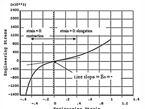
𝑐20 as calculated in Buchaillard et al. will be used: 1037 Pa. and 486 Pa. Figure 7 shows the stress strain relationship derived the Yeoh strain-energy function.

Figure 7: Yeoh second order stress/strain curve acquired from Buchaillard (2007) 22_{the dotted line is the young’s modulus at low}

strains. Stress is measured in Pa.

2.5.2 Active fibre muscles properties (initial model)

In the initial model, muscles are modelled as fibres. Fibres are spring-like structures between elements. When a muscle contracts the tissue properties change; the tissue becomes stiffer. Tissue stiffening due muscle activation in the initial model is simulated by linearly increasing 𝑐10 and 𝑐20 from 1037 Pa. and 486 Pa. with no activation to 10370 Pa. and 4860 Pa. at full activation.

2.5.3 Active element muscle properties (New model)

Because the new model uses element muscles instead of fibre muscles the muscle properties are different. Tissue properties from element muscles in ArtiSynth can change linear with muscle contraction just like the fibre muscles. Another method to simulate the change in tissue stiffness during muscle activation is the method proposed by Blemker et al. (2004)35_. This model includes a dilatational term (Ψ𝑣𝑜𝑙) and deviatoric stress terms that include along-fibre shear (𝑊1), along-fibre stretch (𝑊3) and cross fibre shear (𝑊2).

Ψ = Ψ𝑣𝑜𝑙(𝐽) + 𝑊1(𝛽1) + 𝑊2(𝛽2) + 𝑊3(𝜆, 𝛼)

(3)

With J the relative change in volume and 𝛽1 and 𝛽2 strain invariants which give an independent representation to along-fibre and cross-along-fibre shear36_._𝜆_{is fibre stretch and}_𝛼_{is the} muscle activation level. This active term is added in addition to the passive tissue properties.

2.5.4 Physical simulation – forward modelling

To advance the biomechanical model forward in time physical simulation is needed. At each time step a second-order ordinary differential equation (ODE), that is a result of the physics of the mechanical system, needs to be solved. FEM models in ArtiSynth use lumped mass models as these are easy to connect to rigid bodies or mass-spring (e.g. muscle fibre bundles) components. The formula used is newton’s second law:

𝐌𝐮̇ = 𝐟(𝐪, 𝐮, t) (4)

With 𝐌 the composite mass matrix, 𝐪 the positions of the dynamic components, 𝐮 the velocities, 𝐟(𝐪, 𝐮, t) the force of all force effector components and t the time. Constraints are needed to solve the equations. Bilateral constraints include rigid body joints, FEM incompressibility, and point-surface constraints. Unilateral constraints include contact and joint limits. Equation 4 is integrated using a semi-implicit integrator. Other integrators are also available (Appendix E). This leads to the following linear system for determining the velocities for the next time step.

(𝑴̂ −𝑮𝑇

𝑮 0 ) (𝑼

𝑘+1

𝝀 ) = (

𝑴𝒖𝑘_{+ ℎ𝒇̂}

𝒈 ) (5)

𝑼𝑘+1_{are the velocities for the next time step,}_𝑴_̂ _{is the mass} matrix, 𝒇̂ is the force matrix, h is the time step size, 𝑮 is the matrix of bilateral constrains, 𝝀 are the impulses that enforce constrains and 𝒈 is a term derived from 𝑮̇.

2.5.5 Physical simulation – inverse modelling

[image:11.612.50.295.386.571.2]

(12)

Page | 6 a criterion is needed to come to a single solution. In this case, a

“cost function” is used. This means, in this specific case, that the muscle combination with the lowest combined muscle excitations has to be found. More information details can be found in Appendix E.

2.6 Selection method

Selecting the resection area is the first step of virtual surgery. This only involves the surface mesh (see Figure 8). The primary goal of the selection method is to select the 3D resection area in the most user friendly way. This is difficult because this area has to be 3D. The use of 2D slices to draw the selection area where evaluated but were considered to be too time consuming. More futuristic approaches using virtual reality and a 3D cutting tool would be difficult to get. The best option seemed to be a point and click approach directly on the virtual model. The basic idea is that a selection area will be created by designating corner points of this area. With each click the selection area will be expanded with one corner point. The selection area is automatically closed by connecting the first and last corner point, and will be updated with each mouse click (Figure 9). The only condition is that the corner points are selected in the right order.

Figure 9: Principle of the selection method in 2D. The numbers refer to mouse-clicks.

However, Figure 9 is a 2D drawing and the tongue model is 3D. The interface of ArtiSynth is a 2D representation of a 3D object, in this case the tongue model. The user is looking at the tongue model from a certain angle. This is called the camera angle. When the user clicks at a location on the 2D screen a ray is cast at that point with the same angle as the camera. The objects that this ray encounters with each mouse click are the faces from the surface mesh (see section 2.2.1 ). After clicking, the faces will

be flagged as “selected”. For the selection method not every face that the ray encounters is a valid option for selection. To prevent the selection of faces on the opposite side of the tongue model the standard selection method in ArtiSynth had to be changed. Only the faces that are closest to the camera are selected. The centroid (midpoint of the face) of the faces will act as “corner point” for the drawing method. When more than two faces are selected it is possible to create an area as presented in Figure 9. Because the user must be able to turn the camera while selecting, ray-casting cannot be used to create the selection area (yellow area in Figure 9). Instead a 3D nonvisible area (made visible in Figure 10) is constructed as the user is selecting points. This will be done as follows:

After each mouse click on the model do : For each selected face (i) do:

 Calculate centroid.

 C_up(i) = A point 1 mm* above the centroids of each face, in the direction of the normal.

 C_down(i) = A point 1 mm* below the centroids of each face, in the opposite direction of the normal.

For all selected faces:

 Calculate the mean centroid of all selected faces

 M_up = A point 1 cm* above the mean centroid of all selected faces, in the direction of the normal.

 M_down = A point 1 cm* below the mean centroid of all selected faces, in the opposite direction of the normal.

For each selected face (i) do:

 Create vertices using C_up(i), C_down(i) and C_up(i+1)

 Create vertices using C_up(i+1), C_down(i) and C_up(i+1)

 Create vertices using C_up(i) + C_up(i+1) and M_up

 Create vertices using C_down(i) + C_down(i+1) and M_down

 Create last vertices using the i’th points and the first points.

*The number is not relevant, it has to be elevated above or beneath the selected faces.

(13)

Page | 7

Figure 10: The grey object that is created to cover all faces that are selected.

The resulting (grey) 3D object is presented in Figure 10. Using a built-in function from ArtiSynth all faces within this object can be found. For every face on the surface mesh the centroid coordinates will be calculated. The function searches for the nearest face of the 3D object and determines if the normal of this plane is pointing away or towards the centroid of the specific face on the surface mesh. If the normal points towards the inspected centroid its considered “outside the 3D object “. As long as there are no holes in the surface mesh this function works well. What’s left is an area of selected faces. After the selection of this area, the software not only needs to visualise the surface of the resection but also the depth and shape. When the user selects more than three points, the selected area has to be turned into a volumetric representation of the resection. To create a volumetric representation, the border of the selected area needs to be found. A built-in function can be used to identify all the edges of the border of the selected area. Border edges are only attached to one selected face instead of two. All vertices Pv(i) connected to these border edges will be saved. Using the vertices and there centre point 𝐏𝒄 (average of all vertices) the volumetric representation of the resection shown in Figure 11 is made.

Figure 11: volumetric representation of the resection.

For now we are ignoring the red line. All the structures originating from the border vertices converge to the centre point. In between the vertices and the centre points are also newly created points: The halfway point (𝑷ℎ𝑤(𝑖)).These points can be dynamically adjusted in 2 directions: in the direction of the normal (n) and perpendicular to the normal of the surface area (Figure 12).

Figure 12: A topdown view of the volumetric representation of a virtual resection. Green: center point. Can only move in the direction of the normal. Red: half waypoints. Can move in the direction of the normal and in the direction of the centre point.

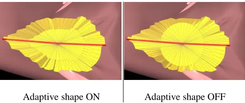
For this last adjustment the adjusted distance can be proportional to the shape of the resection or the absolute distance (Figure 13). This option, called adaptive shape, can be set on or off in the control panel (Figure 14). The centre point

(𝐏𝒄) can only move in the direction of the normal and only relative to 𝑷ℎ𝑤(𝑖). First the centre point 𝐏𝒄 and the deep centre point 𝐏𝒅𝒄 will be calculated:

𝐏𝒅𝒄= (𝐷ℎ𝑤∗ 𝒏) + 𝑪 (6)

𝐏𝒄= ((

𝐷ℎ𝑤

2 ∗ 𝐷𝑐) ∗ 𝒏) + 𝑪

(7)

With 𝐷ℎ𝑤 = depth of halfway points (adjusted with slider on the control panel), 𝐷𝑐 = depth of centre point (adjust with slider), n = normal, C = centroid of selected vertices.

For i = border vertices:

𝑷ℎ𝑤(𝑖)∗= (𝐏𝒗(𝒊)+ 𝐏𝒅𝒄)/2 (8)

Calculate directional vector 𝑽𝑥𝑦𝑧(𝑖) from 𝑷𝒄 to 𝑷ℎ𝑤(𝑖)∗ Calculate distance 𝑉𝑑(𝑖) between 𝑷𝒄and 𝑷ℎ𝑤(𝑖)∗ If adapt shape = true:

𝑷ℎ𝑤(𝑖)= 𝐏𝒄+ ( 𝑽𝑥𝑦𝑧(𝑖)∗ (𝐷𝐶𝐹∗ 𝑉𝑑(𝑖)) ) (9) If adapt shape = false:

[image:13.612.346.533.139.288.2]

(14)

[image:14.612.47.297.53.158.2]

Page | 8

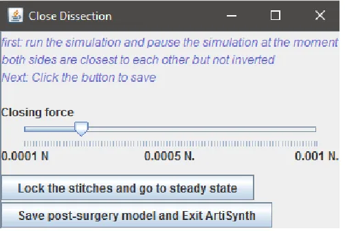
Figure 14: Control panel for surgery tool.

𝐏𝒅𝒄 will only be used to calculate 𝑷ℎ𝑤(𝑖)∗ which is the precursor of 𝑷ℎ𝑤(𝑖) and will only be used to calculate 𝑽𝑥𝑦𝑧(𝑖) and 𝑽𝑑(𝑖). This step is essential to create the cone-like shapes shown in Figure 15. 𝐷𝐶𝐹 is the distance from the centre point to the halfway points. 𝐷𝐶𝐹, 𝐷𝑚𝑝, and 𝐷𝑐 can all be changed with sliders on the control panel (see Figure 14).

This method appeared to be the most flexible and versatile way to select the location for a resection. The main advantage is that it cannot only create a hole but also an almost clear cut. By using the sliders on the control panel almost every shape can be created. Each time the input of a slider changes the method will instantly refresh the volumetric representation so that the user gets real time feedback.

2.7 Removal of tissue and implementation of muscle

At this moment the model consists of a surface mesh, a selected area on the surface mesh and a volumetric representation of the resection (see Figure 8). Vertices from the surface mesh corresponding with the vertices of the volumetric representation are also known. All corresponding faces and vertices from the selected area on the surface mesh except the ones on the edge will be deleted. By merging the corresponding vertices of the volumetric representation and the rest of the surface mesh the perioperative surface mesh is created. Using the same technique for constructing a FEM model as explained in “the new model” a new FEM is generated according to the new shape of the surface mesh. Using the coordinates of the muscle fibres from the initial model in ArtiSynth, muscles fibres can be placed inside the new FEM model (Figure 4). Muscles will only be placed if they are inside the mesh, so they will not be placed inside the resection. As will be explained in section 2.9, these fibres are not sufficient for the simulation of muscle contraction in the new model. They are, however, useful to transfer information about the changed muscle morphology due to the closing of the resection.

Adaptive shape ON Adaptive shape OFF

Figure 13: Sample of a volumetric representation of the resection to show the difference with and without the adapted shape method.

Dc= small

Dhw = normal

DCF = normal

Dc = small

Dhw = large

DCF = normal

Dc = large

Dhw = large

DCF= normal

Dc = large

Dhw = normal

DCF = large

[image:14.612.79.267.207.537.2]

(15)

[image:15.612.49.300.371.539.2]

Page | 9

Figure 16: Illustration of the mechanism behind suturing of the model. Point forces are attached to vertices (black dots). These point forces are pulling the vertices towards the aim on the red plane.

Figure 17: Visual representation of suturing with the surgery tool.

Figure 18: With the slider on the control panel the force that is generated in the point forces can be altered.

2.8 Closing the resection area

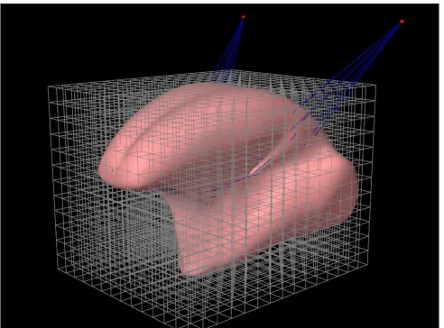
The main reason for splitting the surface mesh and the FEM model was the ability to implement the suturing of the resection. The most obvious way to close the wound would be to steer opposite points on the edge, on either side of the resection, towards each other. This is done using a point force; a force on a certain point in the FEM model. Because of the flexible way the volumetric representation of the resection is selected it is not known how many edge points there are, where they are located, and how they are ordered. Its therefore not always possible to detect opposite edge points. Instead, suturing will be simulated using point forces on the edge of the resection that move towards a (red) plane that is a cross section over the

largest diameter in the resection (Figure 16). The red line, visible in Figure 11, represents the future suture line, and thus the location of the plane. There is a hinge structure halfway the plane to deal with more complex shapes. For each edge point on either side of the plain the projection, and thus target point, on the plain is calculated. The target point on the plain will then be corrected for the distance between the edge point and the centre point of the resection (A + B in Figure 16). This target point on the plain will be their target for the corresponding edge point. As can be seen in Figure 16 this method ensures that there will be as less as possible airspace left in the resection area. The target point on the plane will be levelled with the height of the near target points from the opposite sides (red and green points). In this way, when the resection is closed the opposite sides will be aligned.

When the simulation is started the edge point will slowly move towards there corresponding target point on the plane (see Figure 17). The forces will automatically be lowered exponentially when an edge point reaches there target point on the plane. Using a slider the user can adjust the global force manually (see Figure 18). As individual points forces will be lowered individually, increasing global force will have more effect on edge points with a larger distance from their target. A slider is also needed because different types of resections require different forces in order to close properly.

The drawback of using a plane is that the edge points of the resection (and thus other tongue tissue) are pulled towards a position on a plane that is not necessarily the “rest state” of the sutured tissue. Without dealing with this, the tissue could be pulled to a unnatural position. The last step ensures that the tongue tissue will move to a natural position. When both sides of the resection are close enough the user can “lock” the stitches so that edge points that are close to each other are fixed. The length of these stitches are fixed but the endpoints still have 3 degrees of freedom. When the forces are removed the tongue will return to a steady state where the stresses on the stitch are equally distributed.

At this moment, the FEM model, the surface mesh, and muscle fibres are changed in shape. There is no method available to fix both resection sides in the FEM model without distorting the whole FEM. Therefore, the FEM is removed and only the postoperative muscle locations and the surface mesh are saved (Figure 8). Using this mesh a new FEM structure can be created later the same way as described in section 2.4. Also the location of the resection will be saved to determine the volumetric area in which scar tissue is present later on. Using MeshLab the remaining hole in the mesh is closed.

2.9 Motion simulation

(16)

Page | 10 FEM model is generated, muscle fibre endpoints are not located

on the same spots as nodes anymore. The simulation would still work as the forces would be distributed automatically over the nearest nodes at an endpoint. The movement however would be unnatural. Elements that are in between elements containing a muscle fibre would get squeezed and are not actively involved in muscle contraction. This is not realistic and therefore not desirable. To overcome this problem a method is used to convert the fibre muscles to element muscles. Elements muscles can squeeze themselves and thus act as muscle parts. Elements have different mechanical properties which are described in section 2.5.3 . Information about the position and direction of fibre muscles is used to convert normal elements to muscle elements. Elements that are within a diameter of four millimetre around a certain fibre are converted to element muscles with the same properties. A diameter of four millimetre ensures that most element muscle volumes are comparable with the FEM-muscle version of the initial tongue model (see section 2.3). The muscle forces in the element muscles now have the same direction as the nearby fibre muscles.

Using the information about the location of the resection, fibrosis (scar tissue) is added to the model. Not much is known about the exact extent of the fibrosis and the change in tissue properties of this location. Therefore a method, comparable with stiffening of tissue as part of the free-flap reconstruction approach in Buchaillard (2007)22_{, is used. Different amounts of} stiffness will be used to simulate the stiffening at the former resection location (section 2.11). Also the volume in which the stiffness occurs will be varied in size to inspect the effects.

2.10Validation by comparison with the initial model

First the parameters of the initial model will be compared with the new model. Parameters include: volume of the mesh, volume of the FEM model, number of elements and volume of individual muscle bundles. To compare the motion characteristics of the new model the displacement of the tip of the tongue, after an excitation of 0.3 (1 is maximum contraction) for each muscle, will be compared with the initial model. For this comparison the new model with size factor 200, 300 and 400 will be used.

2.11Validation using patient cases

The initial model cannot be considered as the gold standard because it has never been validated using a patient study. So even more important than the comparison with the initial model will be the simulation of real patient cases. Therefore, pre and postoperative motion data from patients included in the ongoing study of van Dijk et al.24_{will be used. Using the surgery tool} the surgical resections of three patients are imitated. This is done on the basis of pre and postoperative drawings of the surgeon.

2.11.1 Range of Motion measurement

In the study of van Dijk et al.24_{a validated method using 3D} camera is used to measure the range of motion pre and postoperative15_{. Range of Motion (ROM) is expressed in the} Euclidean distance between the tooth gap of the front teeth

(interdental papilla) and the tongue during a manoeuvre. These manoeuvres are: protrusion, left, right, elevation and depression.

Inclusion criteria:

Subjects (ages ranging from 18 to 90 years) undergoing partial glossectomy.

Exclusion criteria:

- Patients that are not able to fill in questionnaires - Palliative treatment

- History of oral cancer treatment - Radiotherapy on tongue surface

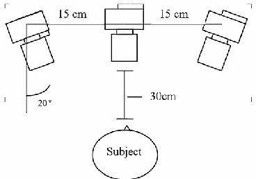
The 3D camera system consists of 3 camera’s fixed in an angle of 20 degrees with a distance of 15 cm to each other. The cameras are then calibrated using an object consisting of 27 beads that are arranged on a 3x3x3 orthogonal grid15_{. For the} information on tongue position reference points are placed on the tongue, the tip of the nose, between the eyes and 2 on the midline of the eyes (see Figure 19 and Figure 20).

Figure 19: Illustration of camera setup used during the ROM measurements.

[image:16.612.345.529.303.432.2]

(17)

Page | 11 2.11.2 Forward simulation

Using inverse modelling the levels of muscle excitations that are needed for the manoeuvres: protrusion, left, right, elevation and depression are determined using a preoperative tongue model. These excitation are then used as input for the postoperative model of a specific patient. The difference between the initial position and the end position in a fixed direction will be the measure of tongue ROM in this research. A fixed direction means that the direction is fixed on the x, y or z axis. This will be compared to the difference between pre and postoperative motion of the three patients. To simulate the effect of scar tissue (or fibrosis), the tissue properties in the resection will be changed. Because the range of change is not known, different configurations will be used:

- no fibrosis

- 12x stiffness, 7 diameter around the initial wound - 12x stiffness, 14 diameter around the initial wound - 14x stiffness, 7 diameter around the initial wound An increase in stiffness is defined as both 𝑐10 and 𝑐20 (see section 2.5.1 ) multiplied x times. These multiplication factors are chosen because “12x stiffness with 7 diameter” gave motion impairment percentages comparable to the ROM measurements of real patients. Other multiplication factors and diameters are omitted for the sake of clarity. This is decided on the basis of manual inspection of ROM measurements and simulations with the biomechanical model. No training set has been used to find the combination that is closest to the ROM measurements.

2.11.3 Inverse simulation

When the human body is exposed to a new situation, the body will try to adapt by compensating. With or without the help of a speech pathologist the patient can train himself to use other muscles to get (nearly) the same movements. This is, however, limited to what is possible with the new postoperative anatomy of the tongue. Using inverse modelling, postoperative models will be forced to find a way to perform a certain manoeuvre. These movements will also be compared with the real patient cases. Only 12x stiffness with a diameter of 7 diameter around the wound is used. In forward modelling this is the setting that is most comparable to the ROM measurements. Additional configurations of the inverse simulation have no added value for this stage of research.

2.11.4 Video inspection

In the results and discussion it will become clear that the Euclidean distance from the ROM measurement is not the best method to validate the biomechanical model. The video inspection is added to compare the forward and inverse simulation directly with the visual inspection of the recorded video. This visual inspection is done solely by the author of this report to give a qualitative measure to compare the biomechanical model with.

3.RESULTS 3.1 Initial model versus new model.

Table 2 shows a comparison of basic properties between the initial model and the new model using a size factor of 200, 300 and 400. The nodes and elements after elimination are showing the amount of nodes and elements left after deleting those which were not inside the surface mesh. It is obvious that the model with size factor 200 has an amount of elements that equals the initial model. Therefore this model simulates movement very quick. However it can be noted that the volume of this FEM model is larger in comparison to the models with size factor 300 and 400. The higher the size factor of the FEM model (and thus amount of elements) the more comparable the volume is to the volume of the surface mesh. There is no volume difference for the surface mesh and FEM model of the initial model as the surface mesh is of the same shape as the FEM model.

Table 2: Volumes of the FEM Models and Surface meshes and the amount of element for and after elimination.

Initial Model

F 200 (15x14x12)

F 300 (23x20x18)

F 400 (31x36x24)

Nodes at start: 947 2912 9576 21600

Elements at start: 739 2340 8280 19344

Nodes after elimination:

1654 4776 9862

Elements after elimination:

1186 3735 8096

Volume of Mesh in cm3

102.29 108.47 108.47 108.47

Volume of FEM in cm3

102.29 157.85 143.09 133.06

[image:17.612.53.293.53.326.2]

(18)

Page | 12 Table 3 shows the volume of each muscle in the initial model

and the new model with size factor 200, 300 and 400. The initial model, in this case, is the FEM muscle version of the initial model. This is because the fibre muscle model uses fibres, and fibres do not have a volume. The FEM muscle version of the initial model is made in such a way that it closely resembles the forces from the initial fibre model.

[image:18.612.131.486.172.733.2]

In order to get comparable motions in the new model, muscles have to match the volume of the initial model almost completely. With fibres converted to elements with a diameter of four millimetre around the fibre (see section 2.7) high volume muscles are matched almost completely. But even after diminishing the diameter, the SL and HG muscles remained about four times larger in comparison to the initial model.

Table 3: Volume of muscle bundles in cm3_{and in % of total volume. Displayed are the initial}

tongue model and the factor 200, 300 and 400 version of the new model.

Initial model factor 200 factor 300 factor 400

GGP_L 9.20 9% 15.53 12% 15.48 11% 15.00 11%

GGP_R 9.20 9% 15.16 11% 15.40 11% 14.48 11%

GGM_L 1.8 2% 5.51 4% 6.14 4% 6.06 5%

GGM_R 1.8 2% 5.39 4% 6.14 4% 5.89 4%

GGA_L 2.25 2% 6.01 5% 6.14 4% 6.15 5%

GGA_R 2.25 2% 5.89 4% 5.87 4% 5.96 4%

GH_L 1.96 2% 5.39 4% 4.73 3% 4.52 3%

GH_R 1.96 2% 5.01 4% 4.69 3% 4.39 3%

MH_L 3.34 3% 10.52 8% 9.53 7% 8.37 6%

MH_R 3.34 3% 10.40 8% 9.49 7% 8.32 6%

HG_L 2.97 3% 14.28 11% 15.06 11% 14.62 11%

HG_R 2.97 3% 13.78 10% 15.18 11% 14.39 11%

VER_L 16.59 16% 20.42 15% 21.20 15% 21.46 16%

VER_R 16.59 16% 20.55 15% 21.50 15% 21.43 16%

TRA_L 18.22 18% 26.43 20% 26.65 19% 26.64 20%

TRA_R 18.22 18% 26.06 20% 26.58 19% 26.15 20%

IL_L 2.25 2% 11.78 9% 11.52 8% 11.07 8%

IL_R 2.25 2% 11.78 9% 11.48 8% 11.05 8%

STY_R 2.48 2% 0.00 0% 0.00 0% 0.00 0%

STY_L 2.48 2% 0.00 0% 0.00 0% 0.00 0%

SL_R 8.50* 8% 39.71 30% 34.39 24% 32.94 25%

(19)

[image:19.612.94.518.74.341.2]

Page | 13

[image:19.612.91.520.391.669.2]

Figure 22: Coordinates of the tonguetip in mm. after an excitation gain of 0.3 on a certain muscle. Blue is the original model, Green is the new model with size factor 200, Yellow is the new model with size factor 300.

(20)

Page | 14 The comparison in Figure 21 shows the differences in

Euclidean distance after an excitation of 0.3 on a single muscle. The purpose of this and the next graph is to compare the reaction of the new and initial model after the excitation of a muscle bundle. From the new model only size factor 200 and 300 are used. A size factor of 400 takes up to much time for a single simulation and is therefore not used for simulation of manoeuvres (only during virtual surgery). The smallest differences can be seen between the factor 200 model (Number 1) and the factor 300 model (Number 2), which are consistent in all muscle bundles. It seems that the model with size factor 300 model is better comparable to the initial model than the factor 200 model. The movement of the GH as well as in the SL muscle are significantly higher in the initial model, while those muscles are much more voluminous in the new models. Figure 22 shows the same models and movements but now in 3D coordinates. The factor 200 model only received an excitation of 0.18 on the SL muscle because a gain of 0.3 caused inverted elements in this case. Although movements of the

different models appeared to be almost the same when looking at the Euclidean distance, this graph highlights another aspect. The movement of the initial model after activation of the GG muscle seems to be almost the same as that of the new model. The GH from the initial model has a large movement in the Y direction in comparison with the new model. This same effect can be seen for the SL muscle in the X direction. The movements of the intrinsic muscles VER and TRA are noticeably different from the initial model, while the Euclidian distance is almost the same. Both the GH and VER show a large movement in Z direction in the new model and a large movement in X and Y direction in the old model. Generally, it can be seen that a small difference in Euclidean distance can still be a quite high actual position difference.

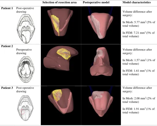
Selection of resection area Postoperative model Model characteristics

Patient 1 Post-operative

drawing Volume difference after

surgery:

In Mesh: 5.77 mm3 _{(5% of} total volume)

In FEM: 7.21 mm3 _{(5% of} total volume)

Patient 2

Preoperative drawing

Volume difference after surgery:

Patient 3 Post-operative drawing

Volume difference after surgery:

[image:20.612.50.562.332.744.2]

(21)

Page | 15 3.2 Patient cases

Three patient cases where included for the validation process. For each patient the pre- and postoperative drawings, the created virtual resections and model characteristics can be found in Table 4. Forward simulations, inverse simulations and the ROM measurements are summarised in one table for each patient (table 5-7). The patient characteristics and video inspection are explained in plain text.

Table 5: Percetages of the differences between the pre and postsurgical final position of the tip of tongue in a certain direction after performing a manouvre.

Patient 1: pre- versus postsurgery Forward simulation

Distance in direction of manoeuvre

protrusion contralateral ipsilateral elevation depression

no fibroses _2% _5% _6% _-5% _11%

12x stiff.

7 diameter 16% 12% 13% 16% 29%

12x stiff.

14 diameter 33% 33% 29% 42% 53%

14x stiff.

7 diameter 21% 17% 36% 24% 35%

Inverse simulation Distance in direction of manoeuvre

protrusion contralateral ipsilateral elevation depression 12x stiff.

7 diameter 16% 6% 4% 0% 24%

Patient ROM measurement Euclidean distance

49% -5% 10% 38% 30%

Patient 1 characteristics

The first patient (57 y/o) was treated for an T1 Squamous cell carcinoma ventral right with unknown amount of affected lymph nodes and zero metastasis (T1NxM0). The diameter of the tumour is 1.8 cm. Because of deep tumour strands there was an additional resection of 4 mm. of the deep edge of the initial resection. The resection volume is 26 mm3_{. As can be seen on} the postoperative drawing in Table 4 a large part of the right anterior and lateral part of the tongue was removed during surgery. The postoperative model shows a tongue, missing many right superficial muscles and a large volume with scar tissue where the wound is closed.

Video Inspection

Postoperative, there is a clear deviation to the ipsilateral side while protruding. The patient cannot elevate the tongue anymore. Before surgery this was about 1 cm. While pointing the tonguetip to the ipsilateral side the reach is about 1 cm less. The largest impairment can be seen while depressing the tongue. Then the range is about 4 cm less.

Patient ROM measurement

Presented in Table 5 are the percentage differences in Euclidian distance of a manoeuvre pre- and postoperative. The patient ROM measurement gives a largely comparable result with the video inspection. But as this is the Euclidian distance, the

protrusion could be under- or overestimated because the tongue was moving to the ipsilateral side too. The impairment while depressing the tongue seemed larger on the video than in the ROM measurements.

Forward simulation

Presented in Table 5 are the percentage difference between the movement in a given direction (not the Euclidian distance) pre and postoperative. With no fibrosis there is almost no change in pre- and postoperative movement. With 12x increased tissue stiffness over a diameter of 7mm around the former resection area the differences become larger. As the exact postoperative properties are unknown, the best setting for fibrosis remains difficult to estimate. Comparable with the video inspection and the patient ROM measurements is that ipsilateral deviation is larger than the contralateral deviation. Also the deviation in depression, which is larger than most other impairments, is comparable with the video inspection. The impairment while protruding is larger in the ROM measurement than in the forward simulation. However it can be seen that in the video inspection the tongue moved to the ipsilateral side while protruding and thus probably gives a overestimation.

Inverse simulation

[image:21.612.44.300.211.433.2]

In the inverse simulation the same impairment can be seen while protruding, but the other impairments are certainly less. The impairment to the ipsilateral side is slightly larger in this case which is not in line with the forward simulation and ROM measurements. Also elevation shows no impairment at all versus 16% in the comparable forward simulation. There are apparently other muscles in this model that can be used to move the tip of the tongue to the same position.

Table 6: percetages of the differences between the pre and postsurgical final position of the tip of tongue in a certain direction after performing a manouvre.

no fibroses _4% _-3% _4% _-6% _2%

12x stiff.

7 diameter 15% 14% 11% 2% 13%

12x stiff.

14 diameter 31% 34% 30% 28% 42%

14x stiff.

7 diameter 18% 21% 14% 5% 17%

12x stiff.

7 diameter 18% 10% 7% -1% 14%

(22)

Page | 16 Patient 2 characteristics

The second patient (67 y/o) was treated for an T2N0M0 squamous cell carcinoma on the right lateral tongue edge. There was no peri- or postoperative drawing available, so the virtual surgery is based on a preoperative drawing of the tumour location and the written report. The exact dimensions of the resection are not known. The resection volume is 16 mm3_. Video inspection

After surgery there is a small decline of about 5 mm. when protruding and a deviation to the ipsilateral side. When the patients tries to move to the ipsilateral side the tongue depresses almost 40 degrees. Movement to the contralateral side is 1 cm. less in the postoperative situation. Elevation of the tongue is almost not possible preoperatively and looks slightly worse after surgery.

Patient ROM measurement

The patient shows an improvement of 43% in Euclidean distance when protruding. This was clearly not the case in the video inspection. Instead, the tongue pointed into a different direction in the postoperative video. There is also a 7% improvement when moving the tongue to the ipsilateral side. Also this is questionable as video inspection shows that the tongue depresses instead of moving to the ipsilateral side. Postoperatively the patient cannot elevate the tongue above her front teeth so an improvement of 15% is also unlikely. Forward simulation

[image:22.612.45.299.505.726.2]

Looking at the forward simulation, there are no real outliers. The decline in motion is mostly the same using all settings. With a fibroses diameter other than 14 mm the decline in elevation is almost non existing. This is comparable to the video inspection showing no outliers in pre and postoperative differences.

Table 7: percetages of the differences between the pre and postsurgical final position of the tip of tongue in a certain direction after performing a manouvre.

no fibroses _0% _6% _5% _-5% _10%

12x stiff.

7 diameter 2% 10% 4% 2% 15%

12x stiff.

14 diameter 11% 22% 13% 13% 30%

14x stiff.

7 diameter 3% 11% 5% 4% 17%

protrusion contralateral ipsilateral elevation depression 12x stiff.

7 diameter 3% 11% 5% -6% 16%

-32% 30% 10% 30% 7%

The results of the inverse simulation are comparable with the forward simulation. Overall there seems to be no improvement in motion capabilities by using other muscles to get the same movement.

Patient 3 characteristics

The third patient (56 y/o) was treated for a T1N0 squamous cell carcinoma at the right tongue base. The ulcer had a diameter of 5 mm and a depth of 1.5 cm. The volume of the tumour is 13 mm3_.

Video inspection

Protrusion is a little less far but not very different from the preoperative video. The motion to the contralateral side declines about 5 mm while the motion to the ipsilateral side remained the same. There is a huge elevation of the tongue pre and post-operatively and the depression did not change notably. Patient ROM measurement

There are large changes in Euclidian distance in the ROM measurements while there are no large differences at video inspection. The only large difference at video inspection was a decline in motion to the contralateral side and a little decline while protruding. The decline in motion at the contralateral side is also visible in the ROM measurements but the improvement in protrusion is probably not realistic.

Forward simulation

In the forward simulation a decline in motion to the contralateral side is also visible in the “12x stiff 7 diameter” simulation. Depression showed a significant change in motion during the simulation, while this was not noticed at video inspection. The other differences are small, which is comparable to the video inspection

There is no noticeable difference between forward and inverse simulation other than that elevation could be improved somewhat. Elevation is even better than in the preoperative model.

3.3 Patient comparison