This paper is made available online in accordance with
publisher policies. Please scroll down to view the document
itself. Please refer to the repository record for this item and our
policy information available from the repository home page for
further information.
To see the final version of this paper please visit the publisher’s website.
Access to the published version may require a subscription.
Author(s): OLAF SCHENK, MATTHIAS BOLLHOFER, AND RUDOLF A.
ROEMER
Article Title: ON LARGE-SCALE DIAGONALIZATION TECHNIQUES
FOR THE ANDERSON MODEL OF LOCALIZATION
Year of publication: 2006
ON LARGE-SCALE DIAGONALIZATION TECHNIQUES FOR THE ANDERSON MODEL OF LOCALIZATION∗
OLAF SCHENK†, MATTHIAS BOLLH ¨OFER‡, AND RUDOLF A. R ¨OMER§
Abstract. We propose efficient preconditioning algorithms for an eigenvalue problem arising in quantum physics, namely the computation of a few interior eigenvalues and their associated eigenvectors for large-scale sparse real and symmetric indefinite matrices of the Anderson model of localization. We compare the Lanczos algorithm in the 1987 implementation by Cullum and Willoughby with the shift-and-invert techniques in the implicitly restarted Lanczos method and in theJacobi–Davidsonmethod. Our preconditioning approaches for the shift-and-invert symmetric
indefinite linear system are based on maximum weighted matchings and algebraic multilevel incom-pleteLDLTfactorizations. These techniques can be seen as a complement to the alternative idea of
using more complete pivoting techniques for the highly ill-conditioned symmetric indefinite Anderson matrices. We demonstrate the effectiveness and the numerical accuracy of these algorithms. Our numerical examples reveal that recent algebraic multilevel preconditioning solvers can accelerate the computation of a large-scale eigenvalue problem corresponding to the Anderson model of localization by several orders of magnitude.
Key words. Anderson model of localization, large-scale eigenvalue problem, Lanczos algo-rithm,Jacobi–Davidsonalgorithm, Cullum–Willoughby implementation, symmetric indefinite
ma-trix, multilevel preconditioning, maximum weighted matching
AMS subject classifications. 65F15, 65F50, 82B44, 65F10, 65F05, 05C85
DOI.10.1137/050637649
1. Introduction. One of the hardest challenges in modern eigenvalue computa-tion is the numerical solucomputa-tion of large-scale eigenvalue problems, in particular those arising from quantum physics such as, e.g., the Anderson model of localization (see section 3 for details). Typically, these problems require the computation of some eigenvalues and eigenvectors for systems which have up to several million unknowns due to their high spatial dimensions. Furthermore, their underlying structure involves random perturbations of matrix elements which invalidates simple preconditioning approaches based on the graph of the matrices. Moreover, one is often interested in finding some eigenvalues and associated eigenvectors in the interior of the spec-trum. The classical Lanczos approach [51] has led to eigenvalue algorithms [16, 17] that are, in principle, able to compute these eigenvalues using only a small amount of memory. More recent work on implicitly restarted Lanczos techniques [42] has accelerated these methods significantly, yet to be fast one needs to combine this ap-proach with shift-and-invert techniques; i.e., in every step one has to solve a shifted system of typeA−σI, where σis a shift near the desired eigenvalues andA∈Rn,n,
∗Received by the editors August 5, 2005; accepted for publication (in revised form) January 31,
2006; published electronically June 19, 2006. This work was supported by the Swiss Commission for Technology and Innovation (CTI) under grant 7036 ENS-ES and by the EPSRC under grant EP/C007042/1.
http://www.siam.org/journals/sisc/28-3/63764.html
†Department of Computer Science, University of Basel, Klingelbergstrasse 50, CH-4056 Basel,
Switzerland ([email protected]).
‡Department of Mathematics, MA 4-5, TU Berlin, Str. des 17. Juni, 10623 Berlin, Germany
([email protected]). The work of this author was supported by the DFG research center
Matheon“Mathematics for Key Technologies” in Berlin.
§Centre for Scientific Computing and Department of Physics, University of Warwick, Coventry
CV4 7AL, UK ([email protected]).
A = AT is the associated matrix. In general, shift-and-invert techniques converge
rather quickly, which is in line with the theory [51]. Still, a linear solver is required to solve systems (A−σI)x=b efficiently with respect to time and memory. While implicitly restarted Lanczos techniques [42] usually require the solution of the system (A−σI)x =b to maximum precision, and thus are mainly suited for sparse direct solvers, the Jacobi–Davidsonmethod has become an attractive alternative [61], in particular when dealing with preconditioning methods for linear systems.
Until recently, sparse symmetric indefinite direct solvers were not as efficient as symmetric positive definite solvers, and this might have been one major reason why shift-and-invert techniques were not able to compete with traditional Lanczos techniques [27], in particular because of memory constraints. With the invention of fast matchings-based algorithms [49], which improve the diagonal dominance of linear systems, the situation has dramatically changed and the impact on precondi-tioning methods [7], as well as the benefits for sparse direct solvers [58], has been recognized. Furthermore, these techniques have been successfully transferred to the symmetric case [22, 24], allowing modern state-of-the-art direct solvers [57] to be orders of magnitudes faster and more memory efficient than ever, finally leading to symmetric indefinite sparse direct solvers that are almost as efficient as their sym-metric positive definite counterparts. Recently this approach has also been utilized to construct incomplete factorizations [38] with similar dramatic success. For a detailed survey on preconditioning techniques for large symmetric indefinite linear systems, the interested reader should consult [5, 6].
2. Numerical approach for large systems. In the present paper we combine the above mentioned advances with inverse-based preconditioning techniques [8]. This allows us to find interior eigenvalues and eigenvectors for the Anderson problem several orders of magnitudes faster than traditional algorithms [16, 17] while still keeping the amount of memory reasonably small.
Let us briefly outline our strategy. We will consider recent novel approaches in preconditioning methods for symmetric indefinite linear systems and eigenvalue problems and apply them to the Anderson model. Since the Anderson model is a large-scale sparse eigenvalue problem in three spatial dimensions, the eigenvalue solvers we deal with are designed to compute only a few interior eigenvalues and eigenvectors, thus avoiding a complete factorization. In particular we will use two modern eigenvalue solvers, which we will briefly introduce in section 5. The first one is Arpack[42], which is a Lanczos-type method using implicit restarts (cf. section 5.1).
We use this algorithm together with a shift-and-invert technique; i.e., eigenvalues and eigenvectors of (A−σI)−1 are computed instead of those of A. Arpack is used in conjunction with a direct factorization method and a multilevel incomplete factorization method for the shift-and-invert technique.
First, we use the shift-and-invert technique with the novel symmetric indefinite sparse direct solver that is part of Pardiso[57], and we report extensive numerical results on the performance of this method. Section 6 will give a short overview of the main concepts that form thePardisosolver. Second, we useArpackin combination with the multilevel incompleteLUfactorization packageIlupack[9]. Here we present a newindefiniteversion of this preconditioner that is devoted to symmetric indefinite problems and combines two basic ideas, namely (i) symmetric maximum weighted matchings [22, 24] and (ii) inverse-based decomposition techniques [8]. These will be described in sections 6.2 and 8.
Davidsonmethod, in particular the implementationJdbsym[32]. This Newton-type
method (see section 5.2) is used together withIlupack [9]. As we will see in several further numerical experiments, the synergy of both approaches will form an extremely efficient preconditioner for the Anderson model that is memory efficient while at the same time accelerates the eigenvalue computations significantly; i.e., system sizes that resulted in weeks of computing time [27] can now be computed within an hour.
3. The Anderson model of localization. The Anderson model of localization is a paradigmatic model describing the electronic transport properties of disordered quantum systems [41, 54]. It has been used successfully in amorphous materials such as alloys [52], semiconductors, and even DNA [53]. Its hallmark is the prediction of a spatial confinement of the electronic motion upon increasing the disorder—the so-called Andersonlocalization [2]. When the model is used in three spatial dimensions, it exhibits a metal-insulator transition in which the disorder strength w mediates a change of transport properties from metallic behavior at smallwvia critical behavior at the transitionwcto insulating behavior and strong localization at largerw[41, 54]. Mathematically, the quantum problem corresponds to a Hamilton operator in the form of a real symmetric matrixA, with quantum mechanical energy levels given by the eigenvalues {λ}, and the respective wave functions are simply the eigenvectors of A, i.e., vectors x with real entries. With N = M ×M ×M sites, the quantum mechanical (stationary) Schr¨odinger equation is equivalent to the eigenvalue equation Ax=λx, which in site representation reads as
xi−1;j;k+xi+1;j;k+xi;j−1;k+xi;j+1;k+xi;j;k−1+xi;j;k+1+εi;j;kxi;j;k=λxi;j;k,
(3.1)
withi, j, k = 1,2, . . . , M, denoting the Cartesian coordinates of a site. The disorder enters the matrix on the diagonal, where the entriesεi;j;k correspond to a spatially
varying disorder potential and are selected randomly according to a suitable distribu-tion [40]. Here, we shall use the standard box distribudistribu-tionεi;j;k ∈[−w/2, w/2] such
that thewparameterizes the aforementioned disorder strength. Clearly, the eigenval-ues ofAthen lie within the interval [−6−w/2, 6 +w/2] due to the Gershgorin circle theorem. In most studies of the disorder-induced metal-insulator transition,wranges from 1 to 30 [54]. But these values also depend on whether generalizations to random off-diagonal elements [26, 63] (the so-called random-hopping problem), anisotropies [44, 47], or other lattice graphs [36, 60] are being considered.
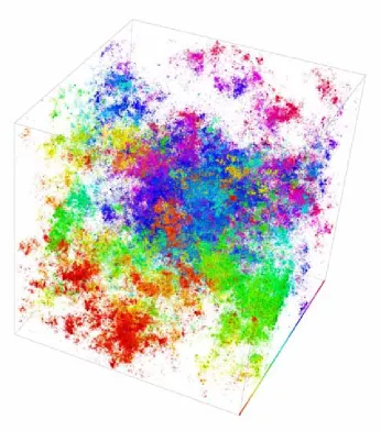
The intrinsic physics of the model is quite rich. For disorders w 16.5, the eigenvectors are extended, i.e.,xi;j;k is fluctuating from site to site, but the envelope |x|is approximately a nonzero constant. For large disordersw >16.5, all eigenvectors are localized such that the envelope|xn|of thenth eigenstate may be approximately written as exp−|r−rn|/ln(w) withr= (i, j, k)T andln(w) denoting thelocalization
length of the eigenstate. In Figure 1, we show examples of such states. Note that
|x|2 and not xcorresponds to a physically measurable quantity and is therefore the observable quantity of interest to physicists. Directly atw=wc ≈16.5, the extended states atλ= 0 vanish and no current can flow. The wave function vectorxappears simultaneously extended and localized, as shown in Figure 2.
Fig. 1. Extended (left) and localized (right) wave function probabilities for the 3D Anderson model with periodic boundary conditions atλ= 0withN= 1003andw= 12.0and21.0, respectively.
Every site with probability|xj|2larger than the average1/N3is shown as a box with volume|xj|2N. Boxes with |xj|2N >
√
1000 are plotted with black edges. The color scale distinguishes between different slices of the system along the axis into the page. The eigenstates have been constructed using Arpackin shift-and-invert mode with Pardisoas a direct solver. See section 9for details.
eigenvectors for the physically most interesting case of critical disorderwc and in the center of σ(A), i.e., at λ= 0, for large system sizes [3, 10, 46, 64]. Since there is a high density of states for σ(A) at λ= 0 in all cases, we have the further numerical challenge of clearly distinguishing the eigenstates in this high density region.
[image:5.612.95.420.102.280.2]4. The Lanczos algorithm and the Cullum–Willoughby implementa-tion. Since the mid 1980s, the preferred numerical tool for studying the Anderson matrix and computing a selected set of eigenvectors, e.g., as needed for a multi-fractal analysis at the transition, was the Cullum–Willoughby implementation (Cwi) [16, 17, 18] of the Lanczos algorithm. Since both Cwiand the algorithm itself are well known, let us here just briefly recall the algorithm’s main benefits, mostly to define our notation. The algorithm iteratively generates a sequence of orthogonal vectorsvi,i= 1, . . . , K, such thatVKTAVK=TK, withV = [v1, v2, . . . , vK] andTK a
symmetric tridiagonal K×K matrix. The recursionβi+1vi+1 =Avi−αivi−βivi−1 defines the diagonal and subdiagonal entries ofTK,αi=viTAvi, andβi+1=vi+1Avi,
respectively. Its associated (Ritz) eigenvalues and eigenvectors then yield those for theA’s.
TheCwiavoids reorthogonalization of thevi’s and hence is very memory efficient. The sparsity of the matrix A can be used to full advantage. However, one needs to construct many Ritz vectors ofTK, which is computationally intensive. Nevertheless,
in 1999 Cwi was still significantly faster than more modern iterative schemes [27]. The main reason for this surprising result lies in the indefiniteness of the sparse matrixA, which led to severe difficulties with solvers more accustomed to standard Laplacian-type problems.
Fig. 2. Plot of the electronic eigenstate at the metal-insulator transition withλ= 0,w= 16.5, and N = 3503. The box-and-color scheme is as in Figure 1. Note how the state extends nearly everywhere while at the same time exhibiting certain localizedregions of higher |xj|2 values. The eigenstate has been constructed using Ilupack-based Jacobi–Davidson. See section9for details.
instead ofAdirectly. This approach relies on the availability of a fast solution method for linear systems of type (A−σI)x=b. However, the limited amount of available memory allows only for a small number of solution steps, and sparse direct solvers also need to be memory efficient to turn this approach into a practical method.
[image:6.612.84.430.97.489.2]under-lying linear system. From the point of view of linear solvers as part of the eigenvalue computation, modern direct and iterative methods need to inherit the symmetric structure A = AT while maintaining both time and memory efficiency. Symmetric
matching algorithms [22, 24, 57] have significantly improved these methods.
5.1. The shift-and-invert mode of the restarted Lanczos method. The Lanczos method for real symmetric matrices Anear a shiftσis based on computing successively orthonormal vectors [v1, . . . , vk, vk+1] and a tridiagonal (k+ 1)×kmatrix
Tk =
⎛ ⎜ ⎜ ⎜ ⎜ ⎜ ⎜ ⎝
α1 β1
β1 α2 . .. . .. . .. β
k−1 βk−1 αk
βk
⎞ ⎟ ⎟ ⎟ ⎟ ⎟ ⎟ ⎠
≡
Tk
βkeTk
, (5.1)
whereek is thekth unit vector inRk, such that
(A−σI)−1[v1, . . . , vk] = [v1, . . . , vk, vk+1]Tk.
(5.2)
Since only a limited number of Lanczos vectors v1, . . . , vk can be stored, and since
this Lanczos sequence also consists of redundant information about undesired small eigenvalues, implicitly restarted Lanczos methods have been proposed [62, 42] that use implicitly shiftedQR[35], exploiting the small eigenvalues ofTk to remove them
from this sequence without ever forming a single matrix vector multiplication with (A−σI)−1. The new transformed Lanczos sequence
(A−σI)−1[˜v1, . . . ,v˜l] = [˜v1, . . . ,˜vl,v˜l+1] ˜Tl
(5.3)
withlkthen allows one to compute furtherk−l approximations. This approach is at the heart of the symmetric version of Arpack[42].
5.2. The symmetric JACOBI–DAVIDSONmethod. One of the major draw-backs of shift-and-invert Lanczos algorithms is the fact that the multiplication with (A−σI)−1 requires solving a linear system to full accuracy. In contrast to this, Jacobi–Davidson-like algorithms [61] are based on a Newton-like approach to solve
the eigenvalue problem. Like the Lanczos method, the search space is expanded step by step, solving the correction equation
(I−uuT)(A−θI)(I−uuT)z=−r such that z= (I−uuT)z, (5.4)
where (u, θ) is the given approximate eigenpair and r =Au−θu is the associated residual. Then the search space based onVk= [v1, . . . , vk] is expanded by
reorthogo-nalizingzwith respect to [v1, . . . , vk], and a new approximate eigenpair is computed
from the Ritz approximation [Vk, z]TA[Vk, z]. When computing several right
eigen-vectors, the projection I−uuT has to be replaced with I−[Q, u][Q, u]T using the
already computed approximate eigenvectors Q. This ensures that the new approxi-mate eigenpair is orthogonal to those that have already been computed.
The most important part of theJacobi–Davidson approach is to construct an approximate solution for (5.4) such that
andK≈A−θI that allows for a fast solution of the systemKx=b. Here, there is a strong need for robust preconditioning methods that preserve symmetry and efficiently solve sequences of linear systems withK. IfKis itself symmetric and indefinite, then the simplified QMR method [29, 30] using the preconditionerI−uwwTTu
K−1, where Kw = u and the system matrix I−uuT(A−θI), can be used as an iterative
method. Note that here the accuracy of the solution of (5.4) is uncritical until the approximate eigenpair converges [28]. This fact has been exploited inJdbsym[4, 32]. For an overview onJacobi–Davidsonmethods for symmetric matrices see [33].
6. On recent algorithms for solving symmetric indefinite systems of equations. We now report on recent improvements in solving symmetric indefinite systems of linear equations that have significantly changed sparse direct as well as preconditioning methods. One key to the success of these approaches is the use of symmetric matchings, which we review in section 6.2.
6.1. Sparse direct factorization methods. For a long time, dynamic pivoting has been a central tool by which nonsymmetric sparse linear solvers gain stability. Therefore, improvements in speeding up direct factorization methods were limited to the uncertainties that have arisen from using pivoting. Certain techniques, like the column elimination tree [19, 34], have been useful for predicting the sparsity pattern despite pivoting. However, in the symmetric case the situation becomes more complicated since only symmetric reorderings, applied to both columns and rows, are required, and no a priori choice of pivots is given. This makes it almost impossible to predict the elimination tree in a sensible manner, and the use of cache-oriented level-3 BLAS [20, 21] is impossible.
With the introduction of symmetric maximum weighted matchings [22] as an alternative to complete pivoting, it is now possible to treat symmetric indefinite sys-tems similarly to how we treat symmetric positive definite syssys-tems. This allows us to predict fill using the elimination tree [31], and thus allows us to set up the data structures that are required to predict dense submatrices (also known as supernodes). This in turn means that one is able to exploit level-3 BLAS applied to the supern-odes. Consequently, the classical Bunch–Kaufman pivoting approach [12] needs to be performed only inside the supernodes.
This approach has recently been successfully implemented in the sparse direct solver Pardiso [57]. As a major consequence of this novel approach, the sparse indefinite solver has been improved to become almost as efficient as its symmetric positive analogy. Certainly for the Anderson problem studied here,Pardisois about two orders of magnitude more efficient than previously used direct solvers [27]. We also note that the idea of symmetric weighted matchings can be carried over to incomplete factorization methods with similar success [38].
6.2. Symmetric weighted matchings as an alternative to complete piv-oting techniques. Symmetric weighted matchings [22, 24], which will be explained in detail in section 7.2, can be viewed as a preprocessing step that rescales the original matrix and at the same time improves the block diagonal dominance. By this strat-egy, all entries are at most one in modulus, and, in addition, the diagonal blocks are either 1×1 scalarsaii such that |aii|= 1 (in exceptional cases we will haveaii = 0)
or 2×2 blocks
aii ai,i+1 ai+1,i ai+1,i+1
Although this strategy does not necessarily ensure that symmetric pivoting, as in [12], is unnecessary, it is nevertheless likely to waive dynamic pivoting during the factoriza-tion process. It has been shown in [24] that, based on symmetric weighted matchings, the performance of the sparse symmetric indefinite multifrontal direct solver MA57 is improved significantly, although a dynamic pivoting strategy by Duff and Reid [25] was still present. Recent results in [57] have shown that the absence of dynamic piv-oting does not harm the method anymore and that, therefore, symmetric weighted matchings can be considered as an alternative to complete pivoting.
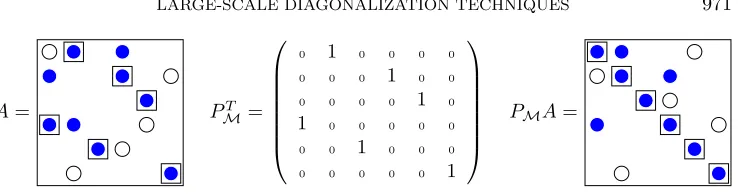
7. Symmetric reorderings to improve the results of pivoting on re-stricted subsets. In this section we will discuss weighted graph matchings as an additional preprocessing step. The motivation for weighted matching approaches is to identify large entries in the coefficient matrix A that, if permuted close to the diagonal, permit the factorization process to identify more acceptable pivots and pro-ceed with fewer pivot perturbations. These methods are based on maximum weighted matchings Mand improve the quality of the factor in a way complementary to the alternative idea of using more complete pivoting techniques. The idea of using a permutationPMassociated with a weighted matchingMas an approximation of the pivoting order for nonsymmetric linear systems was first introduced by Olschowka and Neumaier [49] and extended by Duff and Koster [23] to the sparse case. Permuting the rowsA←PMAof the sparse system to ensure a zero-free diagonal or to maximize the product of the absolute values of the diagonal entries are techniques that are now often regularly used for nonsymmetric matrices [7, 45, 58, 59].
7.1. Matching algorithms for nonsymmetric matrices. LetA = (aij) ∈
Rn×n be a general matrix. The nonzero elements of A define a graph with edges E ={(i, j) : aij = 0} of ordered pairs of row and column indices. A subsetM ⊂ E
is called a matching, or a transversal, if every row index i and every column index j appears at most once in M. A matching M is called perfect if its cardinality is n. For a nonsingular matrix, at least one perfect matching exists and can be found with well known algorithms. With a perfect matching M, it is possible to define a permutation matrixPM= (pij) with
pij =
1 (j, i)∈ M,
0 otherwise. (7.1)
As a consequence, the permutation matrixPMAhas nonzero elements on its diagonal. This method takes only the nonzero structure of the matrix into account. There are other approaches which maximize the diagonal values in some sense. One possibility is to look for a matrix PM such that the product of the diagonal values ofPMAis maximal. In other words, a permutationσhas to be found, which maximizes
n
i=1
|aσ(i)i|. (7.2)
This maximization problem is solved indirectly. It can be reformulated by defining a matrixC= (cij) with
cij=
logai−log|aij| aij = 0,
∞ otherwise,
A= PT M=
⎛ ⎜ ⎜ ⎜ ⎜ ⎜ ⎜ ⎝
0 1 0 0 0 0
0 0 0 1 0 0
0 0 0 0 1 0
1 0 0 0 0 0
0 0 1 0 0 0
0 0 0 0 0 1
⎞ ⎟ ⎟ ⎟ ⎟ ⎟ ⎟ ⎠
PMA=
Fig. 3. Illustration of the row permutation. A small numerical value is indicated by ◦ and a large numerical value by •. The matched entries M are marked with squares, and PM = (e4;e1;e5;e2;e3;e6).
whereai= maxj|aij|, i.e., the maximum element in rowiof matrixA. A permutation
σ, which minimizesni=1cσ(i)i, also maximizes the product (7.2).
The minimization problem is known as the linear sum assignment problem or the bipartite weighted matching problem in combinatorial optimization. The problem is solved by a sparse variant of the Kuhn–Munkres algorithm. The complexity isO(n3) for fulln×nmatrices andO(nτlogn) for sparse matrices withτentries. For matrices whose associated graph fulfills special requirements, this bound can be reduced further to O(nα(τ+nlogn)) with α <1. All graphs arising from difference or
finite-element discretizations meet these conditions [37]. As before, we finally get a perfect matchingMthat in turn defines a nonsymmetric permutationPM.
The effect of nonsymmetric row permutations using a permutation associated with a matchingMis shown in Figure 3. It is clearly visible that the matrix PMA is now nonsymmetric, but has the largest nonzeros on the diagonal.
7.2. Symmetric 1×1 and 2×2 block weighted matchings. In the case of symmetric indefinite matrices, we are interested in symmetrically permutingP APT. The problem is that zero or small diagonal elements of A remain on the diagonal when we use a symmetric permutation P APT. Alternatively, instead of permuting a large1 off-diagonal element aij nonsymmetrically to the diagonal, we can try to
devise a permutation PS such that PSAPST permutes this element close to the diag-onal. As a result, if we form the corresponding 2×2 block to aii aij
aij ajj
, we expect the off-diagonal entryaij to be large, and thus the 2×2 block would form a suitable
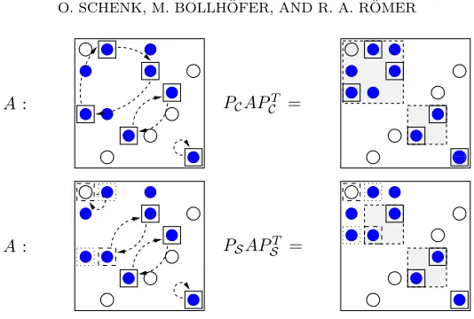
2×2 pivot for the supernode Bunch–Kaufman factorization. An observation on how to build PS from the information given by a weighted matching M was presented by Duff and Gilbert [22]. They noticed that the cycle structure of the permutation PM associated with the nonsymmetric matchingMcan be exploited to derive such a permutation PS. For example, the permutation PM from Figure 3 can be written in cycle representation as PC = (e1;e2;e4)(e3;e5)(e6). This is shown in the upper graphics in Figure 4. The left graphic displays the cycles (1 2 4), (3 5), and (6). If we modify the original permutation PM = (e4;e1;e5;e2;e3;e6) into this cycle permuta-tionPC= (e1;e2;e4)(e3;e5)(e6) and permuteAsymmetrically withPCAPCT, it can be observed that the largest elements are permuted to diagonal blocks. These diagonal blocks are shown by filled boxes in the upper right matrix. Unfortunately, a long cycle would result in a large diagonal block, and the fill-in of the factor for PCAPCT may be prohibitively large. Therefore, long cycles corresponding to PM must be broken down into disjoint 2×2 and 1×1 cycles. These smaller cycles are used to define a symmetric permutationPS = (c1, . . . , cm), wheremis the total number of 2×2 and
[image:10.612.75.444.77.174.2]A: PCAPCT =
00 00 00 11 11 11
A: PSAPT
S =
Fig. 4. Illustration of a cycle permutation with PC = (e1;e2;e4)(e3;e5)(e6) and PS =
(e1)(e2;e4)(e3;e5)(e6). The symmetric matching PS has two additional elements (indicated by dashed boxes), while one element of the original matching fell out (dotted box). The two 2-cycles are permuted into2×2diagonal blocks to serve as initial 2×2pivots.
1×1 cycles.
The rule for choosing the 2×2 and 1×1 cycles fromPC to buildPS is straight-forward. One has to distinguish between cycles of even and odd length. It is always possible to break down even cycles into cycles of length 2. For each even cycle, there are two possible ways to break it down. We use a structural metric [24] to decide which one to take. The same metric is also used for cycles of odd length, but the situation is slightly different. Cycles of length 2l+ 1 can be broken down intol cycles of length 2 and one cycle of length 1. There are 2l+ 1 possible ways to do this. The resulting 2×2 blocks will contain the matched elements of M. However, there is no guarantee that the remaining diagonal element corresponding to the cycle of length 1 will be nonzero. Our implementation will randomly select one element as a 1×1 cycle from an odd cycle of length 2l+ 1.
A selection of PS from a weighted matchingPM is illustrated in Figure 4. The permutation associated with the weighted matching, which is sorted according to the cycles, consists of PC = (e1;e2;e4)(e3;e5)(e6). We now split the full cycle of odd length 3 into two cycles (1)(24)—resulting in PS = (e1)(e2;e4)(e3;e5)(e6). If PS is symmetrically applied to A ← PSAPST, we see that the large elements from the nonsymmetric weighted matchingMwill be permuted close to the diagonal, and these elements will have more chances to form good initial 1×1 and 2×2 pivots for the subsequent (incomplete) factorization.
Good fill-in reducing orderings PFill are equally important for symmetric indef-inite systems. The following section introduces two strategies for combining these reorderings with the symmetric graph matching permutation PS. This will provide good initial pivots for the factorization as well as a good fill-in reduction permutation.
[image:11.612.123.390.75.255.2]Pralet in [24] in order to find good scalings and orderings for symmetric indefinite systems.
In order to combine the permutationPS with a fill-in reducing permutation, we compress the graph of the reordered system PSAPT
S and apply the fill-in reducing
reordering to the compressed graph. In the compression step, the union of the struc-ture of the two rows and columns corresponding to a 2×2 diagonal block is built and used as the structure of a single, compressed row and column representing the original ones.
IfGA= (V;E) is the undirected graph of Aand a cycle consists of two vertices
(s, t) ∈ V, then graph compression will be done on the 1×1 and 2×2 cycles, which have been found using a weighted matching M on the graph. The vertices (s, t) are replaced with a single supervertexu={s, t} ∈Vc in the compressed graph
Gc= (Vc, Ec). An edge ec = (s, t)∈Ec between two superverticess={s1, s2} ∈Vc
andt={t1, t2} ∈Vc exists if at least one of the following edges exists inE: (s1, t1),
(s1, t2), (s2, t1), or (s2, t2). The fill-in reducing ordering is found by applyingMetis on the compressed graphGc = (Vc, Ec). Expansion ofPFillto the original numbering yields the final permutation. Hence all 2×2 cycles that correspond to a suitable 2×2 pivot block are reordered consecutively in the factor.
8. Symmetric multilevel preconditioning techniques. We now present a new symmetric indefinite approximate multilevel factorization that is mainly based on three parts which are repeated in a multilevel framework in each subsystem. The components consist of (i) reordering of the system, (ii) approximate factorization using inverse-based pivoting, and (iii) recursive application to the system of postponed updates.
8.1. Reordering the given system. The key ingredient for turning this ap-proach into an efficient multilevel solver consists of the symmetric maximum weight matching presented in section 6.2. After the system is reordered into a representation
PsTDADPs= ˆA,
(8.1)
where D, Ps ∈ Rn,n, D is a diagonal matrix, and Ps is a permutation matrix, ˆA is
expected to have many diagonal blocks of size 1×1 or 2×2 that are well conditioned. Once the diagonal blocks of size 1×1 and 2×2 are built, the associated block graph of ˆAis reordered by a symmetric reordering, e.g.,Amd[1] orMetis[39], i.e.,
ΠTPsTDADPsΠ = ˜A,
(8.2)
where Π∈Rn,n refers to the associated symmetric block permutation.
8.2. Inverse-based pivoting. Given ˜Awe compute an incomplete factorization LDLT = ˜A+E of ˜A. To do this at stepkof the algorithm we have
˜ A=
B FT
F C =
LB 0
LF I
DB 0
0 SC
LTB LTF
0 I ,
(8.3)
where LB ∈ Rk−1,k−1 is lower triangular with unit diagonal and DB ∈ Rk−1,k−1 is
block diagonal with diagonal blocks of sizes 1×1 and 2×2. Also,SC=C−LFDBLTF =
(sij)i,j denotes the approximate Schur complement. To proceed with the incomplete
Here we use a simple criterion based on block diagonal dominance of the leading block column. Depending on the values
d1=
j>1
|sj1|
|s11|, d2=
j>2
(sj1, sj2)
s11 s12 s12 s22 −1 , (8.4)
we perform a 2×2 update only if d2 < d1. The two leading columns of SC can be
efficiently computed using linked lists [43], and it is not required to have all entries of SC available.
When applying the (incomplete) factorizationLDLT to ˜Awe may still encounter a situation where at step k either 1/|s11| or (sij)−i,j12 is large or even infinite. Since we are dealing with an incomplete factorization we propose to use inverse-based pivoting [8]. Therefore, we require in every step that
LB 0
LF I −1
κ
(8.5)
for a prescribed bound κ. If after the update using a 1×1 pivot (or 2×2 pivot) the norm of the inverse lower triangular factor fails to be less than κ, the update is postponed and the leading rows/columns of LF are permuted to the end of SC.
Otherwise, depending on whether a 1×1 or a 2×2 pivot has been selected, the entries
(sj1/s11)j>1,
(sj1, sj2)
s11 s12 s12 s22 −1 j>2 (8.6)
become the next (block) column of L, and we drop these entries whenever their absolute value is less thanε/κfor some thresholdε. For a detailed description see [8]. The norm of the inverse can be cheaply estimated using a refined strategy of [15] and is part of the software packageIlupack that is now extended to the symmetric indefinite case [9].
8.3. Recursive application. After the inverse-based ILU we have an approxi-mate factorization
QTAQ˜ =
L11 0 L21 I
D11 0 0 S22
LT
11 LT21
0 I ,
(8.7)
and it typically does not pay off to continue the factorization for the remaining matrix S22 which consists of the previously postponed updates. ThusS22 is now explicitly computed and the strategies for reordering, scaling, and factorization are recursively applied toS22, leading to a multilevel factorization.
Note that in order to save memory,L21is not stored but implicitly approximated by ˜A21(L11D11LT11)−1. In addition we use a technique calledaggressive dropping that sparsifies the triangular factorLa posteriori. To do this observe that when applying a perturbed triangular factor ˜L−1 for preconditioning, instead ofL−1we have
˜
L−1= (I+EL)L−1, where EL= ˜L−1(L−L).˜
We can expect that ˜L−1serves as a good approximation toL−1as long asEL 1. If we obtain ˜LfromLby dropping some entry, saylij fromL, then we have to ensure
that
L˜−1ei · |l
for some moderate constant τ <1, e.g.,τ = 0.1. To do this requires having a good estimate for νi ≈ L˜−1ei available for any i = 1, . . . , n. In principle it can be
computed [8, 15] using ˜LT instead of ˜L. Finally, knowing how many entries exist in
columnj, we could drop anylij such that
|lij|τ /(νi·#{lkj: lkj= 0, k=j+ 1, . . . , n}).
8.4. Iterative solution. By construction, the computed incomplete multilevel factorization is symmetric but indefinite. For the iterative solution of linear sys-tems using the multilevel factorization, in principle different Krylov subspace solvers could be used, such as general methods that do not explicitly use symmetry (e.g., GMRES [56]) or methods like SYMMLQ [50] which preserve the symmetry of the original matrix but which are devoted only to symmetric positive definite precondi-tioners. To fully exploit both symmetry and indefiniteness at the same time, here the simplified QMR method [29, 30] is chosen.
9. Numerical experiments. Here we present numerical experiments that show that the previously outlined advances in symmetric indefinite sparse direct solvers as well as in preconditioning methods significantly accelerate modern eigenvalue solvers and allow us to gain orders of magnitude in speed compared to more conventional methods.
9.1. Computing environments and software. All large-scale numerical ex-periments for the Anderson model of localization were performed on an SGI Altix 3700/BX2 with 56 Intel Itanium2 1.6 GHz processors and 112 GB of memory. If not explicitly stated, we always used only one processor of the system and all algorithms were implemented in either C or Fortran77. All codes were compiled by the Intel V8.1 compiler suite using ifort andicc with the−O3 optimization option and linked with basic linear algebra subprograms optimized for Intel architectures. The compu-tations forM = 250,350 andw= 16.5 required 64-bit long integers and−i8 flag for
ifort. From comparison with smaller examples we observed an overhead of approxi-mately 30% with respect to memory and computation time. For completeness, let us recall the main software packages used:
• Arpackis a collection of Fortran77 subroutines designed to solve large-scale eigenvalue problems. The eigenvalue solver has been developed at the De-partment of Computational and Applied Mathematics at Rice University. It is available at http://www.caam.rice.edu/software/ARPACK.
• Jdbsym is a C library implementation of the Jacobi–Davidson method optimized for symmetric eigenvalue problems. It solves eigenproblems of the form Ax=λx and Ax=λBx with or without preconditioning, where Ais symmetric andB is symmetric positive definite. It has been developed at the Computer Science Department of the ETH Z¨urich. It is available at http:// people.web.psi.ch/geus/software.html.
• Pardiso is a fast direct solver package, developed at the Computer Sci-ence Department of the University of Basel. It is available at http://www. computational.unibas.ch/cs/scicomp/software/pardiso.
9.2. CWI compared to shift-and-invert Lanczos with implicit restarts and PARDISO as direct solver. Let us first briefly compare the classical Cwi with the shift-and-invert Lanczos method using implicit restarts. The latter is part of Arpack[42]. For the solution of the symmetric indefinite systemA−θI we use the most recent version of sparse direct solverPardiso[57]. This version is based on symmetric weighted matchings and uses Metis as a symmetric reordering strategy. The numerical results deal with the computation of five eigenvalues of the Anderson matrix A near λ = 0. Here we state the results for the physically most interesting critical disorder strength wc = 16.5. We have measured the CPU times in seconds and memory requirements in GB to compute five eigenvalues closest toλ= 0 of an Anderson matrix of size N = M3×M3 up to M = 100 with Cwi and Arpack– Pardiso. We observe from this initial numerical experiment that the combination of
the shift-and-invert Lanczos with Pardiso is faster when compared to the Cwi by about a factor of 10 for systems with M >50. Despite this success, with increasing problem size the amount of memory consumed by the sparse direct solver becomes significant2 and numerical results withN larger than 1000000 are skipped. Figure 1 shows two different eigenstates computed with the help of Pardiso.
9.3. Using the ILUPACK-based preconditioner. We now switch to the Ilupack-based preconditioner that is also based on symmetric weighted matchings
and in addition uses inverse-based pivoting. In particular, for our experiments we useκ= 5 as a bound for the normL−1 of the inverse triangular factor andAmd for the symmetric reordering. We also tried to use Metis, but for this particular matrix problem we find thatAmdis clearly more memory efficient. Next we compare the shift-and-invert Lanczos (Arpack) withIlupackand the simplified QMR as the inner iterative solver. Here we useε= 1/√N with aggressive dropping, and the QMR method is stopped once the norm of residual satisfiesAx−b10−10b. In order to illustrate the benefits of using symmetric weighted matchings we also triedIlupack without matching, but the numerical results are disappointing, as can be seen from the†’s in Table 9.1. We emphasize that the multilevel approach is crucial; a simple use of incomplete factorization methods without multilevel preconditioning [38] does not give the desired results. Besides the effect of matchings we also compare how the performance of the methods changes when varying the valuew from the critical valuew=wc = 16.5 to w= 12.0 andw= 21.0. We find that these changes do not
affect the sparse direct solver at all while the multilevel ILU significantly varies in its performance. Up to now our explanation for this effect is the observation that with increasing w the diagonal dominance of the system also increases and theIlupack preconditioner gains from higher diagonal dominance. As we can see from Table 9.1, Ilupack still uses significantly less memory than the direct solverPardiso for all
values of w, and it is the only method we were able to use for larger N due to the memory constraints. Also, the computation time is best.
9.4. Using JACOBI–DAVIDSON. When using preconditioning methods inside shift-and-invert Lanczos we usually have to solve the inner linear system for A− θI up to machine precision to make sure that the eigenvalues and eigenvectors are sufficiently correct. In contrast to this the Jacobi–Davidson method allows us to solve the associated correction equation less accurately, and only when convergence takes place is a more accurate solution required. In order to show the significant
2The current standard memory of 2GB RAM for a desktop computer is exceeded for sizes beyond
Table 9.1
CPU times in seconds and memory requirements in GB to compute five eigenvalues closest toλ= 0of an Anderson matrix of sizeM3×M3 with Arpack–Pardiso,Arpack–Ilupack, and Arpack–Ilupack–Symmatch. The symbol — indicates that a memory consumption was larger than
25GB, and †indicates memory problems with respect to the fill-in.
M W Arpack
Pardiso Ilupack Ilupack–Symmatch
Time Mem. Time Mem. Time Mem. 70 12.0 1359 3.00 5117 1.09 2140 0.95 100 12.0 20639 14.34 39222 5.62 13583 3.20
130 12.0 — — † † 65722 8.20
70 16.5 1305 3.00 504 0.33 477 0.31 100 16.5 20439 14.34 2349 0.95 2177 0.89 130 16.5 — — 6320 2.09 6530 1.95 160 16.5 — — 23663 3.95 13863 3.63 70 21.0 1225 3.00 371 0.22 310 0.22 100 21.0 20239 14.34 1513 0.64 1660 0.65 130 21.0 — — 3725 1.41 3527 1.44 160 21.0 — — 15302 2.63 20120 2.68
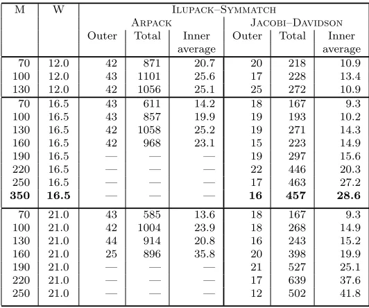
Table 9.2
Number of inner/outer interaction steps inside Arpackand Jacobi–Davidson. The symbol
—indicates that the computations were not performed anymore for Arpack.
M W Ilupack–Symmatch
Arpack Jacobi–Davidson
Outer Total Inner Outer Total Inner average average 70 12.0 42 871 20.7 20 218 10.9 100 12.0 43 1101 25.6 17 228 13.4 130 12.0 42 1056 25.1 25 272 10.9 70 16.5 43 611 14.2 18 167 9.3 100 16.5 43 857 19.9 19 193 10.2 130 16.5 42 1058 25.2 19 271 14.3 160 16.5 42 968 23.1 15 223 14.9
190 16.5 — — — 19 297 15.6
220 16.5 — — — 22 446 20.3
250 16.5 — — — 17 463 27.2
350 16.5 — — — 16 457 28.6
70 21.0 43 585 13.6 18 167 9.3 100 21.0 42 1004 23.9 18 268 14.9 130 21.0 44 914 20.8 16 243 15.2 160 21.0 25 896 35.8 20 398 19.9
190 21.0 — — — 21 527 25.1
220 21.0 — — — 17 639 37.6
250 21.0 — — — 12 502 41.8
difference between the iterative parts of Arpack and Jacobi–Davidson we state the number of iteration steps in Table 9.2. If we were to aim for more eigenpairs, we would expect that eventually theJdbsymwould become less efficient and should again be replaced by Arpack. As stopping criteria for the inner iteration inside the Jacobi–Davidsonmethod we use recent results from [48, 65]. Given the eigenvector
residual
[image:16.612.123.389.343.565.2]and given an approximate solutionzof the correction equation (5.4) with the associ-ated linear system residual
rlin =−reig−(I−uuT)(A−θI)(I−uuT)z,
one could define a new approximate eigenvector via ueignew = (u+z)/u+z.
Fol-lowing [48] the associated new eigenvector residualreignew can be bounded by |rlin −βz|
1 +z2 reignew
(rlin+βz)2+rlin2z2
1 +z2 ,
whereβ =|λ−θ+rT
eigz|. Numerical experiments in [48] indicate that initially
βz rlin ⇒ reignew ≈ rlin 1 +z2,
while asymptotically we expectrlin to converge to zero leading to
βz rlin ⇒ reignew ≈
βz 1 +z2.
Whenz is obtained from the simplified QMR algorithm as in our case, it has been shown in [65] that reignew and rTeigz can be cheaply computed as a by-product of the simplified QMR algorithm. In addition, in practicez need not be recomputed throughout the iteration, since after a few steps,ztypically does not vary too much anymore [48]. This motivates our stopping criterion, where we stop the inner iteration inside QMR whenever
rlin
1 +z2 min
reignew, βz 1 +z2,
τ 2
.
Hereτis the desired tolerance of the eigenvector residual (10−10in our experiments). Note also thatrlinis not explicitly available in the QMR method. Thus we use the quasi residual as an estimate and check only the true residual on exit to safeguard the process.
In what follows we compare the traditional Cwi method with the Jacobi– Davidson code Jdbsym [33] using Ilupack as a preconditioner. Table 9.3 shows
that switching from Arpack to Jacobi–Davidson in this case improves the total time by another factor of 6 or greater. For this reasonJacobi–Davidson together withIlupackwill be used as a default solver in the following. The numerical results in Table 9.3 show a dramatic improvement in the computation time by usingIlupack -basedJacobi–Davidson. Although this new method slows down for smaller wdue to poorer diagonal dominance, a gain by orders of magnitude can still be observed. Forw= 16.5 and larger, even more than three orders of magnitude in the computa-tion time can be observed. Hence the new method drastically outperforms the Cwi method while the memory requirement is still moderate. Figure 2 shows an eigenstate computed within three days with the help of theIlupack-basedJacobi–Davidson. The construction of the Ilupack preconditioner needed 14 hours at a fill-in factor of 18 compared with the fill of the original matrix.
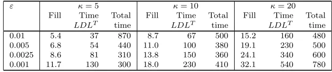
One key to the success of the preconditioner is based on the thresholdκ which bounds the growth ofL−1. Already, for a small example such asM = 70 significant differences can be observed. As we show in Table 9.4, increasing the bound by a factor of 2 fromκ= 5 up toκ= 10 andκ= 20 leads to an enormous increase in fill. Here we measure the fill of the incompleteLDLT factorization relative to the nonzeros of
Table 9.3
CPU times in seconds and memory requirements in GB to compute five eigenvalues closest to
λ= 0withCwiandJacobi–DavidsonusingIlupack–Symmatchfor the shift-and-invert technique.
‡indicates that the convergence of the method was too slow. For Cwiand M = 100, not all five eigenvalues converged successfully, so the eigenvector reconstruction finished more quickly, leading to variances in the CPU times (∗). Computations forM = 250,350, andw= 16.5were computed with 64bit long integers (64).
M W Cwi Jacobi–Davidson
Ilupack–Symmatch
Time Mem. Time Mem. 70 12.0 20228 0.11 1138 0.9 100 12.0 148843 0.32 7238 3.1
130 12.0 ‡ ‡ 52774 9.0
70 16.5 15100 0.11 161 0.3 100 16.5 255842∗ 0.32 661 1.0
130 16.5 ‡ ‡ 2000 2.4
160 16.5 ‡ ‡ 3961 4.8
190 16.5 ‡ ‡ 10955 8.1
220 16.5 ‡ ‡ 25669 12.3
250 16.5 ‡ ‡ 5720364 26.064
350 16.5 ‡ ‡ 18227664 88.064
70 21.0 14371 0.11 99 0.3 100 21.0 331514∗ 0.32 484 0.8
130 21.0 ‡ ‡ 1069 1.6
160 21.0 ‡ ‡ 3070 3.2
190 21.0 ‡ ‡ 8564 5.6
220 21.0 ‡ ‡ 17259 8.5
250 21.0 ‡ ‡ 24802 12.6
Table 9.4
The influence of the inverse bound κon the amount of memory. For M = 70, compare for different thresholds how the fill-innnz(LDLT)/nnz(A)varies depending onκand state the compu-tation time in seconds.
ε κ= 5 κ= 10 κ= 20
Fill Time Total Fill Time Total Fill Time Total
LDLT time LDLT time LDLT time
0.01 5.4 37 870 8.7 67 500 15.2 160 480 0.005 6.8 54 440 11.0 100 380 19.1 230 500 0.0025 8.6 81 310 13.8 150 360 24.1 340 600 0.001 11.7 130 300 18.0 230 410 32.1 540 780
onκis much more significant than the dependence onε. Roughly speaking, the ILU decomposition becomes twice as expensive when κis replaced with 2κ, as does the fill-in. The latter is crucial since memory constraints severely limit the size of the application that can be computed.
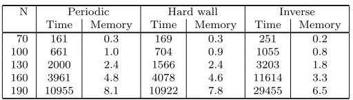
[image:18.612.93.417.436.507.2]Table 9.5
Difference in performance for our standard problem with periodic boundary conditions, the problem with hard wall conditions, and the inverse problem with random numerical entries in the off-diagonal elements. Memory requirement (in GB) and CPU times (in seconds) to compute at the transition the eigenvectors corresponding to the five eigenvalues closest toλ= 0with shift-and-invert Jacobi–Davidsonand theIlupack–Symmatchsolver using symmetric weighted matchings.
N Periodic Hard wall Inverse Time Memory Time Memory Time Memory 70 161 0.3 169 0.3 251 0.2 100 661 1.0 704 0.9 1055 0.8 130 2000 2.4 1566 2.4 3203 1.8 160 3961 4.8 4078 4.6 11614 3.3 190 10955 8.1 10922 7.8 29455 6.5
A to be uniformly distributed in [−1/2,1/2]. The graph of the matrix A remains the same. These values correspond—similarly to wc = 16.5 used before for purely
diagonal randomness—to the physically most interesting localization transition in this model [14]. We note that using hard wall boundary conditions instead of periodic boundary conditions leads to slightly less fill but increases the number of iteration steps, as can be seen in Table 9.5. This conclusions carries over to the off-diagonal Anderson problem, where the memory consumption is less but the iterative part takes even longer. In principle our results could be improved if we were to switch to a smaller thresholdεthan the uniformly appliedε= 1/√N here.
10. Conclusion. We have shown that modern approaches to preconditioning based on symmetric matchings and multilevel preconditioning methods lead to an astonishing increase in performance and available system sizes for the Anderson model of localization. This approach is not only several orders of magnitudes faster than the traditionalCwiapproach, but it also consumes only a moderate amount of memory, thus allowing us to study the Anderson eigenproblem for significantly larger scales than ever before.
Let us briefly recall the main ingredients necessary for this progress. At the heart of the new approach lies the use of symmetric matchings [38] in the precondi-tioning stage of the inverse-based incomplete factorization precondiprecondi-tioning iterative method [9]. Furthermore, the preconditioning itself is of a multilevel type, comple-mentary to the often used full-pivoting strategies. Next, the inverse-based approach is also of paramount importance to keep the fill-in at a manageable level (see Table 9.4). Finally, we emphasize that these results, of course, reflect our selected problem class: to compute a few of the interior eigenvalues and associated eigenvectors for a highly indefinite symmetric matrix defined by the Anderson model of localization.
The performance increase by several orders of magnitude (see Table 9.3) is solely due to our use of new and improved algorithms. Combined with advances in the performance-to-cost ratio of computing hardware during the past six years, current preconditions methods make it possible to solve those problems quickly and easily, which have been considered by far too large until recently [13].
Even forN×N matrices as large as N= 64·106, it is now possible to compute within a few days the interior eigenstates of the Anderson problem.
The success of this method indicates that it might also be successfully applied to other large-scale problems arising in (quantum) physics.
REFERENCES
[1] P. R. Amestoy, T. A. Davis, and I. S. Duff, An approximate minimum degree ordering algorithm, SIAM J. Matrix Anal. Appl., 17 (1996), pp. 886–905.
[2] P. W. Anderson,Absence of diffusion in certain random lattices, Phys. Rev., 109 (1958), pp.
1492–1505.
[3] H. Aoki,Fractal dimensionality of wave functions at the mobility edge: Quantum fractal in the Landau levels, Phys. Rev. B, 33 (1986), pp. 7310–7313.
[4] P. Arbenz and R. Geus,Multilevel preconditioned iterative eigensolvers for Maxwell eigen-value problems, Appl. Numer. Math., 54 (2005), pp. 107–121.
[5] M. Benzi,Preconditioning techniques for large linear systems: A survey, J. Comput. Phys.,
182 (2002), pp. 418–477.
[6] M. Benzi, G. H. Golub, and J. Liesen,Numerical solution of saddle point problems, Acta
Numer., 14 (2005), pp. 1–137.
[7] M. Benzi, J. C. Haws, and M. T˚uma,Preconditioning highly indefinite and nonsymmetric matrices, SIAM J. Sci. Comput., 22 (2000), pp. 1333–1353.
[8] M. Bollh¨ofer and Y. Saad,Multilevel preconditioners constructed from inverse-based ILUs,
SIAM J. Sci. Comput., 27 (2006), pp. 1627–1650.
[9] M. Bollh¨ofer and O. Schenk,ILUPACK Volume 2.0—Preconditioning Software Package for Symmetrically Structured Problems, http://www.math.tu-berlin.de/ilupack/ (2005). [10] T. Brandes, B. Huckestein, and L. Schweitzer,Critical dynamics and multifractal
expo-nents at the Anderson transition in3d disordered systems, Ann. Phys. (Leipzig), 5 (1996), pp. 633–651.
[11] J. R. Bunch,Partial pivoting strategies for symmetric matrices, SIAM J. Numer. Anal., 11
(1974), pp. 521–528.
[12] J. R. Bunch and L. Kaufman,Some stable methods for calculating inertia and solving sym-metric linear systems, Math. Comp., 31 (1977), pp. 163–179.
[13] P. Cain, F. Milde, R. A. R¨omer, and M. Schreiber, Use of cluster computing for the Anderson model of localization, Comput. Phys. Comm., 147 (2002), pp. 246–250. [14] P. Cain, R. A. R¨omer, and M. Schreiber,Phase diagram of the three-dimensional Anderson
model of localization with random hopping, Ann. Phys. (Leipzig), 8 (1999), pp. SI33–SI38. [15] A. K. Cline, C. B. Moler, G. W. Stewart, and J. H. Wilkinson,An estimate for the
condition number of a matrix, SIAM J. Numer. Anal., 16 (1979), pp. 368–375.
[16] J. Cullum and R. A. Willoughby, Lanczos Algorithms for Large Symmetric Eigenvalue Computations, Volume1: Theory, Birkh¨auser Boston, Boston, MA, 1985.
[17] J. Cullum and R. A. Willoughby, Lanczos Algorithms for Large Symmetric Eigenvalue Computations, Volume 2: Programs, Birkh¨auser Boston, Boston, MA, 1985. Available online at http://www.netlib.org/lanczos/.
[18] P. Dayal, M. Troyer, and R. Villiger,The Iterative Eigensolver Template Library, ETH
Z¨urich, Z¨urich, Switzerland, 2004. Available online at http://www.comp-phys.org:16080/ software/ietl/.
[19] J. W. Demmel, S. C. Eisenstat, J. R. Gilbert, X. S. Li, and J. W. H. Liu,A supernodal approach to sparse partial pivoting, SIAM J. Matrix Anal. Appl., 20 (1999), pp. 720–755. [20] D. Dodson and J. G. Lewis,Issues relating to extension of the basic linear algebra
subpro-grams, ACM SIGNUM Newslett., 20 (1985), pp. 19–22.
[21] J. J. Dongarra, J. Du Croz, S. Hammarling, and R. J. Hanson,A proposal for an extended set of Fortran basic linear algebra subprograms, ACM SIGNUM Newslett., 20 (1985), pp. 2–18.
[22] I. S. Duff and J. R. Gilbert, Symmetric weighted matching for indefinite systems, talk
presented at the Householder Symposium XV, 2002.
[23] I. S. Duff and J. Koster,The design and use of algorithms for permuting large entries to the diagonal of sparse matrices, SIAM J. Matrix Anal. Appl., 20 (1999), pp. 889–901. [24] I. S. Duff and S. Pralet,Strategies for Scaling and Pivoting for Sparse Symmetric Indefinite
Problems, Technical Report TR/PA/04/59, CERFACS, Toulouse, France, 2004.
[25] I. S. Duff and J. K. Reid,The multifrontal solution of indefinite sparse symmetric linear equations, ACM Trans. Math. Software, 9 (1983), pp. 302–325.
[26] A. Eilmes, R. A. R¨omer, and M. Schreiber,The two-dimensional Anderson model of local-ization with random hopping, Eur. Phys. J. B, 1 (1998), pp. 29–38.
[28] R. D. Fokkema, G. L. G. Sleijpen, and H. A. Van der Vorst,Jacobi–Davidson style QR and QZ algorithms for the reduction of matrix pencils, SIAM J. Sci. Comput., 20 (1998), pp. 94–125.
[29] R. Freund and F. Jarre,A QMR-based interior-point algorithm for solving linear programs,
Math. Programming Ser. B, 76 (1997), pp. 183–210.
[30] R. Freund and N. Nachtigal,Software for simplified Lanczos and QMR algorithms, Appl.
Numer. Math., 19 (1995), pp. 319–341.
[31] A. George and E. Ng,An implementation of Gaussian elimination with partial pivoting for sparse systems, SIAM J. Sci. Statist. Comput., 6 (1985), pp. 390–409.
[32] R. Geus,JDBSYM Version0.14, http://www.inf.ethz.ch/personal/geus/software.html (2006).
[33] R. Geus, The Jacobi–Davidson Algorithm for Solving Large Sparse Symmetric Eigenvalue Problems with Application to the Design of Accelerator Cavities, Ph.D. thesis, Computer Science Department, ETH Z¨urich, Z¨urich, Switzerland, 2002. Available online at http:// www.inf.ethz.ch/personal/geus/publications/diss-online.pdf.
[34] J. R. Gilbert and E. Ng,Predicting structure in nonsymmetric sparse matrix factorizations,
in Graph Theory and Sparse Matrix Computation, J. A. George, J. R. Gilbert, and J. W. H. Liu, eds., Springer, New York, 1993, pp. 107–139.
[35] G. H. Golub and C. F. Van Loan,Matrix Computations, 3rd ed., The Johns Hopkins
Uni-versity Press, Baltimore, MD, 1996.
[36] U. Grimm, R. A. R¨omer, and G. Schliecker,Electronic states in topologically disordered systems, Ann. Phys. (Leipzig), 7 (1998), pp. 389–393.
[37] A. Gupta and L. Ying,A Fast Maximum-Weight-Bipartite-Matching Algorithm for Reducing Pivoting in Sparse Gaussian Elimination, Tech. Report RC 21576 (97320), IBM T. J. Watson Research Center, Yorktown Heights, NY, 1999.
[38] M. Hagemann and O. Schenk,Weighted matchings for preconditioning symmetric indefinite linear systems, SIAM J. Sci. Comput., 28 (2006), pp. 403–420.
[39] G. Karypis and V. Kumar,A fast and high quality multilevel scheme for partitioning irregular graphs, SIAM J. Sci. Comput., 20 (1998), pp. 359–392.
[40] B. Kramer, A. Broderix, A. MacKinnon, and M. Schreiber,The Anderson transition: New numerical results for the critical exponents, Phys. A, 167 (1990), pp. 163–174. [41] B. Kramer and A. MacKinnon,Localization: Theory and experiment, Rep. Progr. Phys., 56
(1993), pp. 1469–1564.
[42] R. B. Lehoucq, D. C. Sorensen, and C. Yang,ARPACK Users’ Guide: Solution of Large-Scale Eigenvalue Problems with Implicitly Restarted Arnoldi Methods, SIAM, Philadelphia, 1998. Available online at http://www.caam.rice.edu/software/ARPACK/.
[43] N. Li, Y. Saad, and E. Chow,Crout versions of ILU for general sparse matrices, SIAM J.
Sci. Comput., 25 (2003), pp. 716–728.
[44] Q. Li, S. Katsoprinakis, E. N. Economou, and C. M. Soukoulis,Scaling properties in highly anisotropic systems, Phys. Rev. B, 56 (1997), pp. R4297–R4300,
[45] X. S. Li and J. W. Demmel,SuperLU DIST: A scalable distributed-memory sparse direct solver for unsymmetric linear systems, ACM Trans. Math. Software, 29 (2003), pp. 110– 140.
[46] F. Milde, R. A. R¨omer, and M. Schreiber, Multifractal analysis of the metal-insulator transition in anisotropic systems, Phys. Rev. B, 55 (1997), pp. 9463–9469.
[47] F. Milde, R. A. R¨omer, and M. Schreiber, Energy-level statistics at the metal-insulator transition in anisotropic systems, Phys. Rev. B, 61 (2000), pp. 6028–6035.
[48] Y. Notay,Inner Iterations in Eigenvalue Solvers, Technical Report GANMN 05-01, Universit´e
Libre de Bruxelles, Brussels, Belgium, 2005.
[49] M. Olschowka and A. Neumaier,A new pivoting strategy for Gaussian elimination, Linear
Algebra Appl., 240 (1996), pp. 131–151.
[50] C. C. Paige and M. A. Saunders,Solution of sparse indefinite systems of linear equations,
SIAM J. Numer. Anal., 12 (1975), pp. 617–629.
[51] B. N. Parlett, The Symmetric Eigenvalue Problem, Prentice-Hall, Englewood Cliffs, NJ,
1980.
[52] I. Plyushchay, R. A. R¨omer, and M. Schreiber, Three-dimensional Anderson model of localization with binary random potential, Phys. Rev. B, 68 (2003), 064201.
[53] D. Porath, G. Cuniberti, and R. Di Felice, Charge transport in DNA-based devices, in
Long-Range Charge Transfer in DNA II, Topics in Current Chemistry 237, G. B. Schuster, ed., Springer, New York, 2004, p. 183.
[55] Y. Saad,Iterative Methods for Sparse Linear Systems, 2nd ed., SIAM, Philadelphia, 2003.
[56] Y. Saad and M. H. Schultz,GMRES: A generalized minimal residual algorithm for solving nonsymmetric linear systems, SIAM J. Sci. Statist. Comput., 7 (1986), pp. 856–869. [57] O. Schenk and K. G¨artner,On Fast Factorization Pivoting Methods for Symmetric
Indefi-nite Systems, Technical report, Computer Science Department, University of Basel, Basel, Switzerland, 2004. Electron. Trans. Numer. Anal., submitted.
[58] O. Schenk and K. G¨artner,Solving unsymmetric sparse systems of linear equations with PARDISO, J. Future Generation Computer Systems, 20 (2004), pp. 475–487.
[59] O. Schenk, S. R¨ollin, and A. Gupta,The effects of unsymmetric matrix permutations and scalings in semiconductor device and circuit simulation, IEEE Trans. Computer-Aided Design Integrated Circuits Systems, 23 (2004), pp. 400–411.
[60] M. Schreiber and M. Ottomeier,Localization of electronic states in2D disordered systems,
J. Phys.: Condens. Matter, 4 (1992), pp. 1959–1971.
[61] G. L. G. Sleijpen and H. A. Van der Vorst,A Jacobi–Davidson iteration for linear eigen-value problems, SIAM J. Matrix Anal. Appl., 17 (1996), pp. 401–425.
[62] D. C. Sorensen,Implicit application of polynomial filters in ak-step Arnoldi method, SIAM
J. Matrix Anal. Appl., 13 (1992), pp. 357–385.
[63] C. M. Soukoulis and E. N. Economou,Off-diagonal disorder in one-dimensional systems,
Phys. Rev. B, 24 (1981), pp. 5698–5702.
[64] C. M. Soukoulis and E. N. Economou,Fractal character of eigenstates in disordered systems,
Phys. Rev. Lett., 52 (1984), pp. 565–568.