Consistent Induction Motor Parameters for the Calculation of Partial Load Efﬁciencies

(1)

Consistent Induction Motor Parameters for the

Calculation of Partial Load Efficiencies

C. Kral, A. Haumer, and C. Grabner

Abstract—From the rating plate data of an induction motor

the nominal efficiency can be determined. Without detailed knowledge of equivalent circuit parameters, partial load behavior cannot be computed. Therefore, a combined calculation and estimation scheme is presented, where the consistent parameters of an equivalent circuit are elaborated, exactly matching the nominal operating point. From these parameters part load efficiencies can be determined.

Index Terms—Induction motor, consistent parameters, partial

load efficiency

I. INTRODUCTION

T

HE parameter identification and estimation of permanent magnet or [1], [2] electric excited synchronous motors [3], [4], switched reluctance motors [5], [6] and induction mo-tors [7] is essential for various applications. For a controlled drive the performance is very much related with the accuracy of the determined motor parameters [8]–[20], e.g., in energy efficient drives [21], [22]. Another field of applications which may rely on properly determined parameters is condition monitoring and fault diagnosis of electric motors [23]–[25].

For an induction motor, operated at nominal voltage and frequency, and loaded by nominal mechanical power, the current and power factor indicated on the rating plate show certain deviations of the quantities obtained by measurements. The rating plate data are usually rounded and subject to certain tolerances. Deviations of the measured data from the data stated on the rating plate are therefore not surprising.

For the determination of partial load efficiencies of an induction motor, various methods can be applied. One method would be the direct measurement of the electrical and the mechanical power. A second method applies the principle of loss separation; in this case the power balance according to Fig. 2 can be applied. For this purpose it is also required to identify the required motor parameters.

Under some circumstances, it is demanded to determine the partial load efficiency of an induction motor with little or literally no knowledge about the motor. This is a very challenging task, since the full parameter set of an equivalent circuit cannot be computed consistently from the name plate data without further assumptions or knowledge. Practically, one would identify the parameters of the induction motor through several test methods. Thorough investigations of tech-niques for the determination of induction motor efficiencies are presented in [26], [27]. In the presented cases the actual efficiency is analyzed more or less independent of the rating plate data.

In this paper a method for the determination of the con-sistent parameters of the equivalent circuit of an induction

Manuscript received April 8, 2009.

C. Kral, A. Haumer and C. Grabner are with the Austrian Institute of Technology (AIT), business unit Electric Drive Technologies, Giefinggasse 2, 1210 Vienna, Austria (corresponding author to provide phone: +43(5)0550– 6219, fax: +43(5)0550–6595, e-mail: [email protected]).

[image:1.595.329.528.272.338.2]

motor is proposed. In this context it is very important to understand, that the proposed approach does not estimate the parameters of a real induction motor. In this sense, consistent parameters mean, that the determined parameters exactly model the specified operating point specified by the rating plate data summarized in Tab. I.

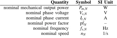
Table I

RATING PLATE DATA OF INDUCTION MOTOR

Quantity Symbol SI Unit

nominal mechanical output power Pm,N W nominal phase voltage Vs,N V nominal phase current It,N A nominal power factor pfN – nominal frequency fs,N Hz

nominal speed nN 1/s

The estimation of motor parameters from name plate data [28]–[30] is thus not sufficient, since the parameters are not implicitly consistent. This means, that the nominal efficiency computed by means of estimated parameters does not exactly compute the nominal operating point.

There are two cases where the determination of consistent parameters is useful. First, a real motor should be investigated, from which, more or less, only the rating plate data are known. Yet partial load efficiencies should be computed for certain operating conditions. Second, the simulation model of an electric drive, which neither has been designed nor built, needs to be parametrized. In such cases, very often only the specification of the nominal operating point is known.

In this paper a calculation for the determination of con-sistent parameters is proposed. The applied model takes stator and rotor ohmic losses, core losses, friction losses and stray-load losses into account, while exactly modeling the specified nominal operating conditions. Some of the required parameters can either be measured, others may be estimated through growth relationships. Due to implicit consistency restrictions, the remaining parameters are solely determined by mathematical equations.

II. POWER ANDTORQUEBALANCE

For the presented power balance and equivalent circuit the following assumptions apply:

• Only three phase induction motors (motor operation) are investigated.

• The motor and the voltage supply are fully symmetrical. • The voltages and currents are solely steady state and of

sinusoidal waveform.

• Only fundamental wave effects of the electromagnetic field are investigated.

• Non-linearities such as saturation and the deep bar effect are not considered.

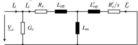
The algorithm presented in this paper relies on the single phase equivalent circuit depicted in Fig. 1. This equivalent

(2)

I′

r

I_t I_s Rs Lsσ L′rσ R′r/s

Lm

Gc

[image:2.595.46.282.37.114.2]

V_s

Figure 1. Equivalent circuit of the induction motor

circuit considers stator and rotor ohmic losses as well as core losses, which is why the phasors of the terminal current I_t and the stator current I_s have to be distinguished.

In order to simplify the explicit calculation of the equivalent circuit parameters, the conductor, representing core losses, is connected directly to the stator terminals. In this approach, stator and rotor core losses

Pc=3GcVs2 (1)

are modeled together, where Gc represents the total core

conductance.

Due to the modeling topology of the equivalent circuit, stator and rotor ohmic losses are

PCus = 3RsIs2, (2)

PCur = 3R′rIr′2. (3)

The rotor parameters of the equivalent circuit are transformed to the stator side, and thus indicated by the superscript′_.

The inner (electromagnetic) power of the motor is deter-mined by

Pi=R′r

1−s

s I

′2

r . (4)

Friction and stray-load losses are not considered in the power balance of the equivalent circuit. Nevertheless, these effects have to be taken into account independently.

Pc PCus PCur Pf Pstray

Ps _P

g _P_i

[image:2.595.42.256.489.619.2]

Pm

Figure 2. Power balance of the the induction motor

In Fig. 2 the total power balance of the motor is depicted. In this balance, the total electrical input power is Ps, and the

air gap power is

Pg=Ps−Pc−PCus. (5)

The inner power

Pi=Pg−PCur (6)

is computed from the inner power and the copper heat losses. Mechanical output (shaft) power

Pm=Pi−Pf−Pstray (7)

is determined from inner power, Pi, friction losses, Pf, and

stray-load losses, Pstray.

Instead of the power balance (7) an equivalent torque balance

τm=τi−τf−τstray, (8)

can be considered. In this context, mechanical output (shaft) torque,τm, is associated with the left side of (7), and the inner

(electromagnetic) torque, τi, is associated with the left side

of (6), etc. Each of these torque terms can be multiplied with the mechanical angular rotor velocityΩm, to obtain equivalent

power terms according to (7).

III. CORE, FRICTION ANDSTRAY-LOADLOSSES

A. Core Losses

For the core loss model hysteresis and eddy current losses have to be taken into account [31]. In a certain operating point the total core losses Pc,ref are known. This operating point refers to a reference voltage Vs,refand the reference frequency fs,ref. Under these conditions a reference conductance can be computed according to

Gc,ref= Pc,ref 3V2

s,ref

. (9)

The ratio of hysteresis losses with respect to the total core losses – with respect to this reference operating point – is ah.

For any other operating point indicated by the actual phase voltage Vs and frequency fs, the total core losses can then be

expressed by

Pc=Pc,ref ah

fs,ref fs

V_s2 V2

s,ref

+ (1−ah)

V_s2 V2

s,ref

!

. (10)

From this relationship the total conductance of the equivalent circuit – as a function of Vs and fs – can be determined:

Gc=Gc,ref

ah

fs,ref fs

+1₋ah

(11)

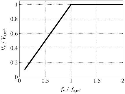
Based on the experience of the authors, it is proposed to set ah≈0.75, if no other estimation is available. In Fig. 3 the

impact of the ratio ahon the total core losses is depicted. The

presented curves are computed for a constant ratio Vs

fs (in the range fs<fs,ref) and constant voltage (in the flux weakening range for fs≥fs,ref) as depicted in Fig. 4.

0 0.5 1 1.5 2

0 0.2 0.4 0.6 0.8 1

fs / fs,ref Pc

/

Pc,

re

f

ah= 0

ah= 0.25

ah= 0.5

ah= 0.75

ah= 1

Figure 3. Total core losses versus frequency; constant Vs

[image:2.595.303.516.585.749.2]

(3)

0 0.5 1 1.5 2 0

0.2 0.4 0.6 0.8 1

fs / fs,ref Vs

/

Vs,

re

[image:3.595.40.256.47.210.2]

f

Figure 4. Voltage versus frequency for inverter operation

B. Friction Losses

The friction losses are modeled by

Pf

Pf,ref =

Ω

m Ωm,ref

af+1

, (12)

(forΩm≥0). In this equation Pf,refandΩm,refare the friction losses and the mechanical angular rotor velocity with respect to a reference operating point, respectively. For axial or forced ventilation af ≈1.5 can be used and radial ventilation can be

modeled by af ≈2.

C. Stray-Load Losses

The stray-load losses are defined as the portion of the total losses in a motor that do not account for stator and rotor ohmic losses, core and friction losses. These losses thus indicate the portion of the losses which can not be calculated. According to the IEEE Standard 112 [32] the percentages astray of the stray-load losses with respect to the nominal output power for the nominal operating point are summarized in Tab. II.

Table II

STRAY-LOAD PERCENTAGES ACCORDING TOIEEE STANDARD112

nominal output power [kW] percentage astray

1–90 0.018

91–375 0.015

376–1850 0.012

greater than 1850 0.009

From the actual terminal current It and the no load terminal

current It,0, the approximated rotor current can be calculated by

I2=

q

I2

t −It2,0. (13)

In the IEEE Standard 112, the stray-load losses are consid-ered by a quadratic dependency of (13). Since the standard does not take any variable frequency dependencies into ac-count, the stray-load loss are proposed to be approximated by

Pstray=astrayPm,N

I_t2₋I_t2_,₀

I2

t,N−It2,0

Ω

m Ωm,N

2

, (14)

which can be considered as an extension to the standard [33]. In [34], the stray-load losses are considered as an equivalent resistor in the equivalent circuit. Since the voltage drop across such a resistor has no physical background, the stray-load losses are modeled differently in this paper: the stray-load

losses are inherently taken into account by an equivalent breaking torque,

τstray=astrayPm,N

I2

t −It2,0 I_t2_,_N−I_t2_,₀

Ωm Ω2

m,N

, (15)

according to (8).

IV. SPACEPHASOREQUATIONS

The space phasor equations of electric machines can be derived based on the definitions of [35]. With respect to the equivalent circuit of Fig. 1, the stator voltage and terminal current space phasor (with respect to the stator fixed reference) frame are

Vs_s = 2

3(vs,1+e j2π/3_v

s,2+e−j2π/3vs,3), (16)

Is_t = 2

3(it,1+e j2π/3_i

t,2+e−j2π/3it,3), (17)

where vs,1, vs,2 and vs,3 are the stator phase voltages, and it,1, it,2 and it,3 are the terminal phase currents, respectively. These space phasors can be transformed into a synchronous reference frame; the angular velocity of this reference frame is

ωs=2πfs. (18)

The reference frame of the transformed stator voltage and terminal current is indicated by a superscript index:

V_sf = Vs_se−j(ωst−ϕf) ₍₁₉₎

I_tf = I_tse−j(ωst−ϕf) (20)

The electrical rotor speed is

ωm=pΩm, (21)

since space phasor theory relies on an equivalent two pole induction motor. The voltage equations with respect to Fig. 1 are





Vsf

0 Vsf



=





0 Rs+jωsLs jωsLm

0 jωrLm Rr+jωrLr

1/Gc −1/Gc 0 

 

 

I_tf Isf

Irf 

 ,

(22) where

ωr=ωs−ωm. (23)

The rotor leakage and main field inductances of the equiv-alent circuit in Fig. 1 and the rotor resistance cannot be determined independently [36]. It is thus useful to introduce the stray factor

σ=1− L

2

m

LsL′r

, (24)

and the ratio of stator to rotor inductance

σsr=

Ls

L′

r

, (25)

as well as the terms

as =

ωsLs

Rs

, (26)

ar = ωr

L′

r

R′

r

. (27)

(4)

The linear set of equations (22) has the solutions

I_sf = V_sf as(1+jar)

ωsLs[1−σasar+j(as+ar)]

, (28)

I_rf = V_sf −j

√

1−σ√σsrasar ωsLs[1−σasar+j(as+ar)]

, (29)

according to [37]. The inner torque yields:

τi=

3p 2

V_s2

ω2

sLs

(1−σ)a2

sar

(1−σasar)2+ (as+ar)2

(30)

It is obvious that (28) and (30) are independent of σsr.

This is an important result, which refutes the myth that for a squirrel cage induction motor the inductance L′

r can be

determined without further assumptions. Yet, the rotor current (29) is certainly dependent on σsr. For the assignment of

specific values to the parameters Lm, L′r and R′r and for the

calculation of the rotor current the arbitrary factorσsr has to

be chosen according to

1−σ≤σsr≤

1

1₋σ. (31)

V. DETERMINATION OFPARAMETERS

In the following a combination of parameter calculations and estimations, based on empirical data, is presented. The presented results all refer to empirical data obtained from 50 Hz standard motors. Unfortunately the empiric data cannot be revealed in this paper. Nevertheless the applied mathemati-cal approach for the estimation is presented. For motors with a certain mechanical power and number of pole pairs empirical data can be approximated with good accuracy.

The determination of the equivalent circuit parameters is, however, based on the rating plate data of the motor (Tab. I). From these data the nominal electrical input power

Ps,N=3Vs,NIt,NpfN (32)

and the nominal angular rotor velocity

Ωm,N=2πnN (33)

can be computed.

A. Measurement or Estimation of Core Losses

If measurement results are obtained from a real motor, the core losses can be determined according to IEEE Standard 122 [32], by separating core and friction losses. The no load core losses, Pc,0, refer to the nominal voltage and nominal frequency. It is assumed that the no load test is performed at synchronous speed (s=0),

Ωm,0= 2πfs,N

p . (34)

In case measurement results are not available, the no load friction losses, for a motor with a certain nominal mechanical output power, Pm,N, and a certain number of pole pairs, p, can

be estimated from empirical data by

log₁₀

_P

c,0 P′

c

=kc[p]log10

_P

m,N

P′

m

+dc[p]. (35)

In this equation, P_c′and P_m′ are arbitrary reference power terms to normalize the argument of the logarithm. The parameters kc[p] and dc[p] are obtained from the empiric data and

par-ticularly refer to a specific number of pole pairs. From the

estimated or measured no load core losses the reference core conductance can be derived according to (9),

Gc,ref= Pc,0 3Vs,N

. (36)

B. Measurement or Estimation of Friction Losses

From a no load test (s=0) the friction losses, Pf,0, of a particular real motor can also be determined. In case no measurements are available, the no load friction losses can be estimated from empirical data,

log₁₀ Pf,0 P′

f !

=k_f_[_p_]log₁₀

_P

m,N

P′

m

+d_f_[_p_]. (37)

In this equation P′

f and Pm′ are some arbitrary reference

power terms, and k_f_[_p_] and d_f_[_p_] are empiric parameters corresponding for a certain number of pole pairs. According to (12), the no load friction losses Pf,0=Pf,refare corresponding withΩm,0=Ωm,ref .

C. Calculation of Stray-Load Losses

The nominal stray load losses can be derived from

Pstray,N=astrayPm,N, (38)

and parameter astray can be obtained by Tab. II.

D. Estimation of Stator Resistance

The stator resistance can be estimated applying the power balance of Fig. 2 with respect to the nominal operation point. From the nominal mechanical output power, Pm,N, the nominal

friction losses

Pf,N=Pf,0

Ω

m,N Ωm,0

af+1

(39)

and the nominal stray-load losses (38), the nominal inner power

Pi,N=Pm,N−Pf,N−Pstray,N (40)

can be calculated. The air gap power can be determined from the nominal inner power and nominal slip, sN [37]:

Pg,N=

Pi,N

1₋sN

(41)

The stator copper losses can then be obtained by the power balance (5), applied to the nominal operating point,

PCus,N=Ps,N−Pg,N−Pc,N. (42)

Since the core loss conductor is connected to the terminals in Fig. 1, the core losses with respect to the nominal and no load operating point are equal,

Pc,N=Pc,0. (43)

From the the nominal stator phase current, and the nom-inal stator copper losses (42) consistent stator resistance are determined by

Rs=

PCu,s,N

3I2

s,N

. (44)

In this equation the nominal stator current, Is,N has to be

determined from (22).

(5)

derived through a numeric iteration. In other words: there are two options on how the stator resistance and the core losses can be determined. Either the stator resistance or the core losses have to be measured or estimated, and the remaining quantity can then be computed by (40)–(44).

E. Measurement or Estimation of No Load Current

In the following space phasor calculations are applied to the nominal operating conditions. The phase angle ϕf of

synchronous reference is chosen such way that the imaginary part of the stator voltage space phasor

V_sf_,_N=Vsx,N+jVsy,N (45)

is zero,

Vsx,N = √

2Vs,N (46)

Vsy,N = 0. (47)

If the no load terminal current

I_tf_,₀=Itx,0+jIty,0 (48)

has not been obtained by measurement results, the reactive component has to be estimated. This can be performed by

log₁₀ Ity,0 I′

ty,0

!

=k₀_[_p_]log₁₀

_P

m,N

P′

m

+d₀_[_p_], (49)

where I′

ty,0 and Pm′ are an arbitrary reference current and

power term. The parameters k₀_[_p_]and d₀_[_p_]are estimated from empiric data with respect to a certain number of pole pairs. Then the imaginary part of the stator current space phasor can be derived by

Isy,0=Ity,0, (50)

according to (48) and (22). Once all the parameters of the motor are determined, the consistent no load current It,0 can be determined from the equivalent circuit, evaluating (14).

F. Determination of Stator Inductance

The rotor current space phasor diminishes under no load conditions, and thus the stator current equation of (22) yields:

√

2Vs,N = RsIsx,0−ωsLsIyx,0 (51) 0 = ωsLsIsx,0+RsIsy,0 (52)

By eliminating the real part, Isx,0, in these equations, the re-maining equation for the imaginary part, considering Isy,0<0, can be used to determine the stator inductance

Ls=−

Vsx,N+ q

V_sx2_,_N₋4R2

sIsy2,0 2ωsIsy,0

. (53)

G. Determination of Stray Factor and Rotor Time Constant

The components of the nominal terminal current space phasor are

I_tf_,_N=Itx,N+jIty,N (54)

From the components of the terminal current

Itx,N = +It,NpfN, (55)

Ity,N = −It,N q

1₋pf2_N, (56)

the components of the stator current space phasor can be derived:

Isx,N = Itx,N− √

2GcVs,N, (57)

Isy,N = Ity,N. (58)

The real and the imaginary part of (28) yields:

Vsx,N

Rs

= (1−σasar)Isx,N−(as+ar)Isy,N (59)

ar

as

Vsx,N

Rs

= (as+ar)Isx,N+ (1−σasar)Isy,N (60)

From these two equations the two unknown parameters

ar =

asRsIs2,N+Isy,NVsx,N

Isx,NVsx,N−RsIs2,N

, (61)

σ = (2Isx,N−asIsy,N)Vsx,N−RsI 2

s,N− V2

sx,N

Rs as(asRsIs2,N+Isy,NVsx,N)

, (62)

can be obtained. The rotor time constant is the ratio of the rotor inductance and the rotor resistance and can be expressed in terms of known parameters, utilizing (27),

Tr=

ar ωr,N

, (63)

whereωr,N refers to the nominal operating point. From (61)–

(63) it can be seen that the rotor time constant and the leakage factor are independent of the particular choice of σsr.

H. Determining Magnetizing Inductance, Rotor Inductance and Rotor Resistance

From the leakage factors σ and σsr, and the stator

in-ductance Ls, utilizing (31), the following equations can be

derived:

Lm = Ls

√

1₋σ

√_σ sr

(64)

L′_r = _σLs

sr

(65)

From (63) and (65) the rotor resistance can be computed.

R′_r=L ′

r

Tr

. (66)

The quantities determined in this subsection are fully depen-dent on the particular choice ofσsr.

VI. MEASUREMENT ANDCALCULATIONRESULTS

Table III

RATING PLATE OF18.5KWMOTOR

Quantity Value

nominal mechanical output power Pm,N=18.5 kW nominal phase voltage Vs,N=400 V

nominal phase current It,N=18.9 A nominal power factor pfN=0.9

nominal frequency fs,N=50 Hz nominal speed nN=1460 rpm

(6)

Table IV

PARAMETERS OF18.5KWMOTOR

Parameter Value

stator resistance Rs=0.4784Ω stator inductance Ls=0.2755 H stray factor σ=0.05683 magnetizing inductance Lm=0.2676 H

rotor inductance Lr=0.2755 H rotor resistance Rr=0.5625Ω core conductance Gc,0=0.0007539 S no load friction losses Pf,0=211.4 W nominal stray-load losses Pstray,N=333.0 W

A. Investigation of a 18.5 kW Motor

A detailed comparison of calculation and measurement results is presented for a 18.5 kW four pole induction motor. In Tab. III the rating plate data of the induction motor are summarized. The investigations are performed for the motor operated at nominal voltage and frequency. Core and friction losses are known from a no load test. The stray load losses are determined according to Tab. II. For this motor the consistent parameters are calculated and summarized in Tab. IV with

[image:6.595.319.538.67.235.2]

σsr=1, ah=0.75, af =1.5, and astray=0.018. The losses corresponding with the nominal operating point are calculated (Tab. V).

Table V

CALCULATED POWER AND LOSSES FOR NOMINAL OPERATION OF

18.5KWMOTOR

parameter value

electrical input power Ps,N=20412 W core losses Pc,N=361.9 W stator ohmic losses PCus,N=498.1 W rotor ohmic losses PCur,N=521.4 W friction losses Pf,N=197.6 W stray-load losses Pstray,N=333.0 W mechanical output power Pm,N=18500 W

In Fig. 5 and 6 the measurement and calculation results of the electrical input and the mechanical output power are compared. The efficiency

η=Pm Ps

(67)

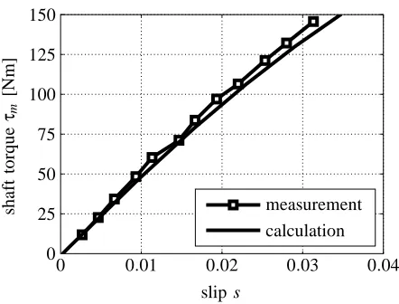
and the power factor are depicted in Fig. 7 and 8. The stator current and the mechanical output torque are shown in Fig. 9 and 10. The validity and usability of the proposed calculation algorithm is demonstrated by the presented measurement and calculation results.

Since the computation of the consistent parameters is based on the rating plate data of the motor, it is not surprising that the nominal operating point (specified by the rating plate) and the measurement results do not exactly coincide. Instead, a higher goal is achieved: the calculations exactly match the specified nominal operating point.

B. Investigation of Motors based on Manufacturer Data

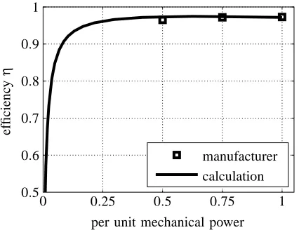
The series of 1.1 kW, 11 kW, 110 kW and 1000 kW induc-tion motors is also investigated in this paper. For each power rating, manufacturer data of motors for p=1, p=2 and p=3 are compared with calculations (and estimations, respec-tively). Apart from the nominal operating point, manufacturer data provide additionally the efficiencies for 75% and 50% of the nominal mechanical output power. In Fig. 11–22 the catalog based manufacturer data and the results obtained from calculations are compared.

0 0.01 0.02 0.03 0.04 0

5 10 15 20 25 30

slip s

el

ec

tr

ic

al

p

o

w

er

Ps

[k

W

]

[image:6.595.86.249.72.168.2]

measurement calculation

Figure 5. Electrical input power versus slip of a four pole induction motor with 18.5 kW; measurement and calculation

0 0.01 0.02 0.03 0.04 0

5 10 15 20 25 30

slip s

m

ec

h

an

ic

al

p

o

w

er

Pm

[k

W

]

Figure 6. Mechanical output power versus slip of a four pole induction motor with 18.5 kW; measurement and calculation

0 0.01 0.02 0.03 0.04 0.5

0.6 0.7 0.8 0.9 1

slip s

ef

fi

ci

en

cy

η

[image:6.595.319.535.319.486.2] [image:6.595.318.538.567.738.2]

(7)

0 0.01 0.02 0.03 0.04 0

0.2 0.4 0.6 0.8 1

slip s

p

o

w

er

fa

ct

o

r

p

f

[image:7.595.322.533.63.225.2]

Figure 8. Power factor versus slip of a four pole induction motor with 18.5 kW; measurement and calculation

0 0.01 0.02 0.03 0.04 0

5 10 15 20 25 30

slip s

te

rm

in

al

cu

rr

en

t

It

[A

]

[image:7.595.56.278.69.234.2]

Figure 9. Terminal current versus slip of a four pole induction motor with 18.5 kW; measurement and calculation

0 0.01 0.02 0.03 0.04 0

25 50 75 100 125 150

slip s

sh

af

t

to

rq

u

e

τm

[N

m

]

Figure 10. Mechanical output torque versus slip of a four pole induction motor with 18.5 kW; measurement and calculation

0 0.25 0.5 0.75 1

0.5 0.6 0.7 0.8 0.9 1

per unit mechanical power

ef

fi

ci

en

cy

η

[image:7.595.322.532.315.480.2]

manufacturer calculation

Figure 11. Efficiency versus per unit mechanical output power for a two pole induction motor with Pm,N=1.1 kW, Vs,N=400 V, Is,N=1.34 A, pfN=0.86,

fs,N=50 Hz and nN=2810 rpm; manufacturer data and calculation

0 0.25 0.5 0.75 1

0.5 0.6 0.7 0.8 0.9 1

ef

fi

ci

en

cy

η

[image:7.595.59.274.319.486.2]

Figure 12. Efficiency versus per unit mechanical output power for a four pole induction motor with Pm,N=1.1 kW, Vs,N=400 V, Is,N=1.48 A, pfN=0.769,

0 0.25 0.5 0.75 1

0.5 0.6 0.7 0.8 0.9 1

ef

fi

ci

en

cy

η

Figure 13. Efficiency versus per unit mechanical output power for a six pole induction motor with Pm,N=1.1 kW, Vs,N=400 V, Is,N=1.66 A, pfN=0.75,

[image:7.595.322.534.566.731.2] [image:7.595.56.277.569.737.2]

(8)

0 0.25 0.5 0.75 1 0.5

0.6 0.7 0.8 0.9 1

ef

fi

ci

en

cy

η

[image:8.595.322.534.62.226.2]

Figure 14. Efficiency versus per unit mechanical output power for a two pole induction motor with Pm,N=11 kW, Vs,N=400 V, Is,N=11.4 A, pfN=0.89,

0 0.25 0.5 0.75 1

0.5 0.6 0.7 0.8 0.9 1

ef

fi

ci

en

cy

η

[image:8.595.62.276.65.226.2]

Figure 15. Efficiency versus per unit mechanical output power for a four pole induction motor with Pm,N=11 kW, Vs,N=400 V, Is,N=12.1 A, pfN=0.84,

0 0.25 0.5 0.75 1

0.5 0.6 0.7 0.8 0.9 1

ef

fi

ci

en

cy

η

Figure 16. Efficiency versus per unit mechanical output power for a six pole induction motor with Pm,N=11 kW, Vs,N=400 V, Is,N=13.2 A, pfN=0.79,

fs,N=50 Hz and nN=876 rpm

0 0.25 0.5 0.75 1

0.5 0.6 0.7 0.8 0.9 1

ef

fi

ci

en

cy

η

[image:8.595.323.532.314.481.2]

Figure 17. Efficiency versus per unit mechanical output power for a two pole induction motor with Pm,N=110 kW, Vs,N=400 V, Is,N=107 A, pfN=0.90,

0 0.25 0.5 0.75 1

0.5 0.6 0.7 0.8 0.9 1

ef

fi

ci

en

cy

η

[image:8.595.62.273.315.480.2]

Figure 18. Efficiency versus per unit mechanical output power for a four pole induction motor with Pm,N=110 kW, Vs,N=400 V, Is,N=110.3 A, pfN= 0.88, fs,N=50 Hz and nN=1485 rpm; manufacturer data and calculation

0 0.25 0.5 0.75 1

0.5 0.6 0.7 0.8 0.9 1

ef

fi

ci

en

cy

η

Figure 19. Efficiency versus per unit mechanical output power for a six pole induction motor with Pm,N=110 kW, Vs,N=400 V, Is,N=116 A, pfN=0.84,

[image:8.595.63.276.565.732.2] [image:8.595.323.534.565.732.2]

(9)

0 0.25 0.5 0.75 1 0.5

0.6 0.7 0.8 0.9 1

ef

fi

ci

en

cy

η

[image:9.595.62.275.64.228.2]

Figure 20. Efficiency versus per unit mechanical output power a for two pole induction motor with Pm,N=1000 kW, Vs,N=3464 V, Is,N=109 A, pfN= 0.91, fs,N=50 Hz and nN=2988 rpm; manufacturer data and calculation

0 0.25 0.5 0.75 1

0.5 0.6 0.7 0.8 0.9 1

ef

fi

ci

en

cy

η

[image:9.595.62.275.310.481.2]

Figure 21. Efficiency versus per unit mechanical output power for a four pole induction motor with Pm,N=1000 kW, Vs,N=3464 V, Is,N=114 A, pfN= 0.87, fs,N=50 Hz and nN=1494 rpm; manufacturer data and calculation

0 0.25 0.5 0.75 1

0.5 0.6 0.7 0.8 0.9 1

ef

fi

ci

en

cy

η

Figure 22. Efficiency versus per unit mechanical output power for a six pole induction motor with Pm,N=1000 kW, Vs,N=3464 V, Is,N=113 A, pfN= 0.88, fs,N=50 Hz and nN=996 rpm; manufacturer data and calculation

VII. CONCLUSIONS

The intention of this paper was the calculation of the consistent parameters of an induction motor. In this context it is important to know that the proposed approach does not model the real motor behavior, but exactly models the nominal operating point, specified by the rating plate. In the presented model ohmic losses, core losses, friction losses and stray-load losses are considered. Mathematical algorithms and estimations – where necessary – are presented. For an investigated four pole 18.5 kW induction motor, measurement and calculation results are compared, revealing well matching results and thus proving the applicability of the presented calculations. Additionally, the manufacturer data of a series of two, four and six pole motors in the range of 1.1 kW to 1000 kW are compared with calculations. Even for these mo-tors the obtained manufacturer data show that the calculations are very well matching.

APPENDIX

NOMENCLATURE Variables

a abbreviation; factor d term of approximation

ϕ phase angle

G reluctance

i instantaneous current

I RMS current

I current phasor k term of approximation

L inductance

p number of pole pairs P power, losses pf power factor

Ψ flux linkage

Ψ flux linkage phasor

R resistance

σ leakage factor

s slip

T time constant

τ torque

v instantaneous voltage

V RMS voltage

V voltage phasor

ω electrical angular velocity

Ω mechanical angular velocity

Indexes

0 no load operation 1,2,3 phase indexes

c core

Cu copper

e eddy current losses f friction losses

g air gap

h hysteresis losses

i inner

m magnetizing; mechanical (rotor) N nominal operation

[image:9.595.63.274.566.732.2]

(10)

r rotor

s stator

sr stator and rotor stray stray-load losses

t terminal

x real part, with respect to a synchronous ref-erence frame

y imaginary part, with respect to a synchronous reference frame

Superscripts

f synchronous reference frame s stator fixed reference frame

∗ conjugate complex

′ _{with respect to the stator side; reference}

REFERENCES

[1] J.-Y. Lee, S.-H. Lee, G.-H. Lee, J.-P. Hong, and J. Hur, “Determination of parameters considering magnetic nonlinearity in an interior perma-nent magnet synchronous motor,” IEEE Transactions on Magnetics, vol. 42, no. 4, pp. 1303–1306, April 2006.

[2] M. Kondo, “Parameter measurements for permanent magnet syn-chronous machines,” Transactions on Electrical and Electronic

Engi-neering IEEJ Trans 2007, vol. 109-117, 2007.

[3] M. Burth, G. C. Verghese, and M. Velez-Reyes, “Subset selection for improved parameter estiamtion on on-line identification on a syn-chronous generator,” IEEE Transactions on Power Systems, vol. 14, no. 1, pp. 218–225, 1999.

[4] E. Kyriakides, G. Heydt, and V. Vittal, “Online parameter estimation of round rotor synchronous generators including magnetic saturation,”

IEEE Transactions on Energy Conversion, vol. 20, no. 3, pp. 529–537,

Sept. 2005.

[5] S. Ichikawa, M. Tomita, S. Doki, and S. Okuma, “Sensorless control of synchronous reluctance motors based on extended emf models considering magnetic saturation with online parameter identification,”

IEEE Transactions on Industry Applications, vol. 42, no. 5, pp. 1264–

1274, Sept.-Oct. 2006.

[6] P. Niazi and H. A. Toliyat, “Online parameter estimation of permanent-magnet assisted synchronous reluctance motor,” IEEE Transactions on

Industry Applications, vol. 43, no. 2, pp. 609–615, March-april 2007.

[7] R. Babau, I. Boldea, T. J. E. Miller, and N. Muntean, “Complete parameter identification of large induction machines from no-load acceleration–deceleration tests,” IEEE Transactions on Industrial

Elec-tronics, vol. 54, no. 4, pp. 1962–1972, Aug. 2007.

[8] R. F. F. Koning, C. T. Chou, M. H. G. Verhaegen, J. B. Klaassens, and J. R. Uittenbogaart, “A novel approach on parameter identification for inverter driven induction machines,” IEEE Transactions on Control

Systems Technology, vol. 8, 6, pp. 873–882, 2000.

[9] J.-K. Seok and S.-K. Sul, “Induction motor parameter tuning for high-performance drives,” IEEE Transactions on Industry Applications, vol. 37, no. 1, pp. 35–41, 2001.

[10] H. Tajima, G. Guidi, and H. Umida, “Consideration about problems and solutions of speed estimation method and parameter tuning for speed-sensorless vector control of induction motor drives,” IEEE Transactions

on Industry Applications, vol. 38, No. 5, pp. 1282–1289, 2002.

[11] C. Grantham and D. J. McKinnon, “Rapid parameter determination for induction motor analysis and control,” IEEE Transactions on Industry

Applications, vol. 39, no. 4, pp. 1014–1020, July-August 2003.

[12] R. Wamkeue, I. Kamwa, and M. Chacha, “Unbalanced transients-based maximum likelihood identification of induction machine parameters,”

IEEE Transactions on Energy Conversion, vol. 18, no. 1, pp. 33–40,

March 2003.

[13] H. A. Toliyat, E. Levi, and M. Raina, “A review of rfo induction motor parameter estimation techniques,” IEEE Transactions on Energy

Conversion, vol. 18, no. 2, pp. 271–283, June 2003.

[14] M. Cirrincione, M. Pucci, G. Cirrincione, and G.-A. Capolino, “A new experimental application of least-squares techniques for the estimation of the induction motor parameters,” IEEE Transactions on Industry

Applications, vol. 39, No. 5, pp. 1247–1256, 2003.

[15] ——, “Constrained minimization for parameter estimation of induction motors in saturated and unsaturated conditions,” IEEE Transactions on

Industrial Electronics, vol. 52, no. 5, pp. 1391–1402, Oct. 2005.

[16] A. Boglietti, A. Cavagnino, and M. Lazzari, “Experimental high-frequency parameter identification of ac electrical motors,” IEEE

Trans-actions on Industry Applications, vol. 43, no. 1, pp. 23–29, Jan.-feb.

2007.

[17] H. Kobayashi, S. Katsura, and K. Ohnishi, “An analysis of parameter variations of disturbance observer for motion control,” IEEE

Transac-tions on Industrial Electronics, vol. 54, no. 6, pp. 3413–3421, Dec.

2007.

[18] A. B. Proca and A. Keyhani, “Sliding-mode flux observer with online rotor parameter estimation for induction motors,” IEEE Transactions on

Industrial Electronics, vol. 54, no. 2, pp. 716–723, April 2007.

[19] D. P. Marcetic and S. N. Vukosavic, “Speed-sensorless ac drives with the rotor time constant parameter update,” IEEE Transactions on Industrial

Electronics, vol. 54, no. 5, pp. 2618–2625, Oct. 2007.

[20] S. Maiti, C. Chakraborty, Y. Hori, and M. C. Ta, “Model reference adap-tive controller-based rotor resistance and speed estimation techniques for vector controlled induction motor drive utilizing reactive power,”

IEEE Transactions on Industrial Electronics, vol. 55, no. 2, pp. 594–

601, Feb. 2008.

[21] A. Mirecki, X. Roboam, and F. Richardeau, “Architecture complexity and energy efficiency of small wind turbines,” IEEE Transactions on

Industrial Electronics, vol. 54, no. 1, pp. 660–670, Feb. 2007.

[22] D. de Almeida Souza, W. C. P. de Aragao Filho, and G. C. D. Sousa, “Adaptive fuzzy controller for efficiency optimization of induction motors,” IEEE Transactions on Industrial Electronics, vol. 54, no. 4, pp. 2157–2164, Aug. 2007.

[23] X.-Q. Liu, H.-Y. Zhang, J. Liu, and J. Yang, “Fault detection and diagnosis of permanent-magnet dc motor based on parameter estimation and neural network,” IEEE Transactions on Industrial Electronics, vol. 47, no. 5, pp. 1021–1030, Oct. 2000.

[24] C. Kral, R. Wieser, F. Pirker, and M. Schagginger, “Sequences of field-oriented control for the detection of faulty rotor bars in induc-tion machines—the vienna monitoring method,” IEEE Transacinduc-tions on

Industrial Electronics, vol. 47, no. 5, pp. 1042–1050, October 2000.

[25] S. Bachir, S. Tnani, J. C. Trigeassou, and G. Champenois, “Diagnosis by parameter estimation of stator and rotor faults occurring in induction machines,” IEEE Transactions on Industrial Electronics, vol. 53, no. 3, pp. 963–973, June 2006.

[26] J. Hsu, J. Kueck, M. Olszewski, D. Casada, P. Otaduy, and L. Tolbert, “Comparison of induction motor field efficiency evaluation methods,”

IEEE Transactions on Industry Applications, vol. 34, no. 1, pp. 117–

125, Jan.-Feb. 1998.

[27] B. Lu, T. Habetler, and R. Harley, “A survey of efficiency-estimation methods for in-service induction motors,” IEEE Transactions on

Indus-try Applications, vol. 42, no. 4, pp. 924–933, July-August 2006.

[28] H. König, “Ermittlung der Parameter der Drehstrom-Asynchronmaschine vorwiegend aus den Typenschildangaben,”

Elektrie, vol. 6, pp. 220–220, 1988.

[29] J. Pedra and F. Corcoles, “Estimation of induction motor double-cage model parameters from manufacturer data,” IEEE Transactions

on Energy Conversion, vol. 19, no. 2, pp. 310–317, June 2004.

[30] K. Davey, “Predicting induction motor circuit parameters,” IEEE

Trans-actions on Magnetics, vol. 38, no. 4, pp. 1774–1779, July 2002.

[31] D. Lin, P. Zhou, W. Fu, Z. Badics, and Z. Cendes, “A dynamic core loss model for soft ferromagnetic and power ferrite materials in transient finite element analysis,” Conference Proceedings COMPUMAG, 2003. [32] “IEEE standard test procedures for polyphase induction motors and

generators,” IEEE Standard 112, 2004.

[33] W. Lang, “Über die Bemessung verlustarmer Asynchronmotoren mit Käfigläufer für Pulsumrichterspeisung,” Ph.D. dissertation, Technische Universität Wien, 1984.

[34] P. Pillay, V. Levin, P. Otaduy, and J. Kueck, “In-situ induction motor ef-ficiency determination using the genetic algorithm,” IEEE Transactions

on Energy Conversion, vol. 13, no. 4, pp. 326–333, Dec. 1998.

[35] P. K. Kovacs, Transient Phenomena in Electrical Machines. Budapest: Akademiai Kiado Verlag, 1984.

[36] H. Kleinrath, “Ersatzschaltbilder für Transformatoren und Asynchron-maschinen,” e&i, vol. 110, pp. 68–74, 1993.