Improved Natural Language Learning via
Variance-Regularization Support Vector Machines
Shane Bergsma University of Alberta [email protected]
Dekang Lin Google, Inc. [email protected]
Dale Schuurmans University of Alberta [email protected]
Abstract
We present a simple technique for learn-ing better SVMs uslearn-ing fewer trainlearn-ing ex-amples. Rather than using the standard SVM regularization, we regularize toward low weight-variance. Our new SVM ob-jective remains a convex quadratic func-tion of the weights, and is therefore com-putationally no harder to optimize than a standard SVM. Variance regularization is shown to enable dramatic improvements in the learning rates of SVMs on three lex-ical disambiguation tasks.
1 Introduction
Discriminative training is commonly used in NLP and speech to scale the contribution of different models or systems in a combined predictor. For example, discriminative training can be used to scale the contribution of the language model and translation model in machine translation (Och and Ney, 2002). Without training data, it is often rea-sonable to weight the different models equally. We propose a simple technique that exploits this intu-ition for better learning with fewer training exam-ples. We regularize the feature weights in a Sup-port Vector Machine (Cortes and Vapnik, 1995) to-ward a low-variance solution. Since the new SVM quadratic program is convex, it is no harder to op-timize than the standard SVM objective.
When training data is generated through hu-man effort, faster learning saves time and money. When examples are labeled automatically, through user feedback (Joachims, 2002) or from tex-tual pseudo-examples (Smith and Eisner, 2005; Okanohara and Tsujii, 2007), faster learning can reduce the lag before a new system is useful.
We demonstrate faster learning on lexical dis-ambiguation tasks. For these tasks, a system pre-dicts a label for a word in text, based on the
word’s context. Possible labels include part-of-speech tags, named-entity types, and word senses. A number of disambiguation systems make pre-dictions with the help of N-gram counts from a web-scale auxiliary corpus, typically via a search-engine (Lapata and Keller, 2005) or N-gram cor-pus (Bergsma et al., 2009). When discriminative training is used to weigh the counts for classifi-cation, many of the learned feature weights have similar values. Good weights have low variance.
For example, consider the task of preposition selection. A system selects the most likely prepo-sition given the context, and flags a possible error if it disagrees with the user’s choice:
• I worked in Russia from 1997 to 2001.
• I worked in Russia *during 1997 to 2001.
Bergsma et al. (2009) use a variety of web counts to predict the correct preposition. They have fea-tures for COUNT(in Russia from), COUNT(Russia
from 1997),COUNT(from 1997 to), etc. If these are
high, from is predicted. Similarly, they have fea-tures for COUNT(in Russia during), COUNT(Russia
during 1997), COUNT(during 1997 to). These
fea-tures predict during. All counts are in the log domain. The task has thirty-four different prepo-sitions to choose from. A 34-way classifier is trained on examples of correct preposition usage; it learns which context positions and sizes are most reliable and assigns feature weights accordingly.
A very strong unsupervised baseline, however, is to simply weight all the count features equally. In fact, in Bergsma et al. (2009), the supervised approach requires over 30,000 training examples before it outperforms this baseline. In contrast, we show that by regularizing a classifier toward equal weights, a supervised predictor outperforms the unsupervised approach after only ten exam-ples, and does as well with 1000 examples as the standard classifier does with 100,000.
Section 2 first describes a general multi-class SVM. We call the base vector of information used by the SVM the attributes. A standard multi-class SVM creates features for the cross-product of attributes and classes. E.g., the attribute
COUNT(Russia during 1997) is not only a feature
for predicting the preposition during, but also for predicting the 33 other prepositions. The SVM must therefore learn to disregard many irrelevant features. We observe that this is not necessary, and develop an SVM that only uses the relevant attributes in the score for each class. Building on this efficient framework, we incorporate variance regularization into the SVM’s quadratic program.
We apply our algorithms to three tasks: prepo-sition selection, context-sensitive spelling correc-tion, and non-referential pronoun detection (Sec-tion 4). We reproduce Bergsma et al. (2009)’s results using a multi-class SVM. Our new mod-els achieve much better accuracy with fewer train-ing examples. We also exceed the accuracy of a reasonable alternative technique for increasing the learning rate: including the output of the unsuper-vised system as a feature in the SVM.
Variance regularization is an elegant addition to the suite of methods in NLP that improve perfor-mance when access to labeled data is limited. Sec-tion 5 discusses some related approaches. While we motivate our algorithm as a way to learn better weights when the features are counts from an aux-iliary corpus, there are other potential uses of our method. We outline some of these in Section 6, and note other directions for future research.
2 Three Multi-Class SVM Models
We describe three max-margin multi-class classi-fiers and their corresponding quadratic programs. Although we describe linear SVMs, they can be extended to nonlinear cases in the standard way by writing the optimal function as a linear combi-nation of kernel functions over the input examples. In each case, after providing the general tech-nique, we relate the approach to our motivating application: learning weights for count features in a discriminative web-scale N-gram model.
2.1 Standard Multi-Class SVM
We define aK-class SVM following Crammer and Singer (2001). This is a generalization of binary SVMs (Cortes and Vapnik, 1995). We have a set
{(¯x1, y1), ...,(¯xM, yM)}ofM training examples.
Eachx¯ is anN-dimensional attribute vector, and
y ∈ {1, ..., K}are classes. A classifier, H, maps an attribute vector, x¯, to a class,y. H is parame-terized by aK-by-N matrix of weights,W:
HW(¯x) =argmaxK
r=1
{W¯r·x¯} (1)
whereW¯r is therth row ofW. That is, the
pre-dicted label is the index of the row ofW that has
the highest inner-product with the attributes,x¯. We seek weights such that the classifier makes few errors on training data and generalizes well to unseen data. There are KN weights to learn, for the cross-product of attributes and classes. The most common approach is to train K sep-arate one-versus-all binary SVMs, one for each class. The weights learned for the rth SVM pro-vide the weightsW¯rin (1). We call this approach
OvA-SVM. Note in some settings various one-versus-one strategies may be more effective than one-versus-all (Hsu and Lin, 2002).
The weights can also be found using a single constrained optimization (Vapnik, 1998; Weston and Watkins, 1998). Following the soft-margin version in Crammer and Singer (2001):
min
W,ξ1,...,ξM
1 2
K
X
i=1
||W¯i||2+C m
X
i=1
ξi
subject to : ξi≥0
∀r 6=yi, W¯yi ·x¯i−W¯r·x¯i≥1−ξi (2)
The constraints require the correct class to be scored higher than other classes by a certain mar-gin, with slack for non-separable cases. Minimiz-ing the weights is a form of regularization. TunMinimiz-ing theC-parameter controls the emphasis on regular-ization versus separation of training examples.
We call this the K-SVM. The K-SVM out-performed the OvA-SVM in Crammer and Singer (2001), but see Rifkin and Klautau (2004). The popularity ofK-SVMis partly due to convenience; it is included in popular SVM software like SVM
-multiclass1andLIBLINEAR(Fan et al., 2008). Note that with two classes, K-SVM is less effi-cient than a standard binary SVM. A binary classi-fier outputs class 1 if (w¯·x >¯ 0) and class 2 other-wise. TheK-SVMencodes a binary classifier using
¯
W1= ¯wandW¯2=−w¯, therefore requiring twice
the memory of a binary SVM. However, both bi-nary and 2-class formulations have the same solu-tion (Weston and Watkins, 1998).
1
2.1.1 Web-Scale N-gramK-SVM
K-SVMwas used with N-gram models in Bergsma et al. (2009). For preposition selection, attributes were web counts of patterns filled with 34 preposi-tions, corresponding to the 34 classes. Each prepo-sition serves as the filler of each context pattern. Fourteen patterns were used for each filler: all five 5-grams, four 4-grams, three 3-grams, and two 2-grams spanning the position to be predicted. There areN=14∗34=476total attributes, and therefore
KN =476∗34=16184weights inW.
This K-SVM classifier can potentially exploit very subtle information. Let W¯in and W¯bef ore
be weights for the classes in and before. Notice some of the attributes weighted in the inner prod-uctsW¯bef ore·x¯andW¯in·x¯will be for counts of
the preposition after. Relatively high counts for a context with after should deter us from choosing in more than from choosing before. These cor-relations can be encoded in the classifier via the corresponding weights on after-counts inW¯inand
¯
Wbef ore. How useful are these correlations and
how much training data is needed before they can be learned and exploited effectively?
We next develop a model that, for each class, only scores those attributes deemed to be directly relevant to the class. Our experiments thus empir-ically address these questions for different tasks.
2.2 SVM with Class-Specific Attributes
Suppose we can partition our attribute vectors into sub-vectors that only include attributes that we de-clare as relevant to the corresponding class: x¯ = (¯x1, ...,x¯K). We develop a classifier that only
uses the class-specific attributes in the score for each class. The classifier uses anN-dimensional weight vector,w¯, which follows the attribute par-tition,w¯ = ( ¯w1, ...,w¯K). The classifier is:
Hw¯(¯x) = K
argmax
r=1
{w¯r·¯xr} (3)
We call this classifier the CS-SVM(an SVM with Class-Specific attributes).
The weights can be determined using the follow (soft-margin) optimization:
min
¯
w,ξ1,...,ξm
1 2w¯
Tw¯+C m
X
i=1
ξi
subject to : ξi ≥0
∀r6=yi, w¯yi·x¯iyi −w¯r·x¯ir≥1−ξi (4)
There are several advantages to this formula-tion. Foremost, rather than having KN weights, it can have only N. For linear classifiers, the number of examples needed to reach optimum performance is at most linear in the number of weights (Vapnik, 1998; Ng and Jordan, 2002). In fact, both the total number and number of active features per example decrease byK. Thus this re-duction saves far more memory than what could be obtained by an equal reduction in dimensional-ity via pruning infrequent attributes.
Also, note that unlike theK-SVM(Section 2.1), in the binary case theCS-SVMis completely equiv-alent (thus equally efficient) to a standard SVM.
We will not always a priori know the class as-sociated with each attribute. Also, some attributes may be predictive of multiple classes. In such cases, we can include ambiguous attributes in ev-ery sub-vector (needing N+D(K-1)total weights ifD attributes are duplicated). In the degenerate case where every attribute is duplicated, CS-SVM
is equivalent toK-SVM; both haveKN weights.
2.2.1 Optimization as a Binary SVM
We could solve the optimization problem in (4) directly using a quadratic programming solver. However, through an equivalent transformation into a binary SVM, we can take advantage of effi-cient, custom SVM optimization algorithms.
We follow Har-Peled et al. (2003) in transform-ing a multi-class example into a set of binary examples, each specifying a constraint from (4). We extend the attribute sub-vector corresponding to each class to be N-dimensional. We do this by substituting zero-vectors for all the other sub-vectors in the partition. The attribute vector for the
rth class is thenz¯r= (¯0, ...,¯0,x¯r,¯0, ...,¯0). This is
known as Kesler’s Construction and has a long his-tory in classification (Duda and Hart, 1973; Cram-mer and Singer, 2003). We then create binary rank constraints for a ranking SVM (Joachims, 2002) (ranking SVMs reduce to standard binary SVMs). We createK instances for each multi-class exam-ple (x¯i, yi), with the transformed vector of the true class,z¯yi, assigned a higher-rank than all the other,
equally-ranked classes, z¯{r6=yi}. Training a
rank-ing SVM usrank-ing these constraints gives the same weights as solving (4), but allows us to use effi-cient, custom SVM software.2 Note the K-SVM
2One subtlety is whether to use a single slack,ξi
Us-can also be trained this way, by including every attribute in every sub-vector, as described earlier.
2.2.2 Web-Scale N-gramCS-SVM
Returning to our preposition selection example, an obvious attribute partition for the CS-SVM is to include as attributes for predicting preposition r
only those counts for patterns filled with preposi-tionr. Thusx¯inwill only include counts for
con-text patterns filled with in and ¯xbef ore will only
include counts for context patterns filled with
be-fore. With 34 sub-vectors and 14 attributes in each,
there are only14∗34=476total weights. In con-trast,K-SVMhad16184weights to learn.
It is instructive to compare theCS-SVMin (3) to the unsupervised SUMLM approach in Bergsma et al. (2009). That approach can be written as:
H(¯x) =argmaxK
r=1
{¯1·x¯r} (5)
where¯1is anN-dimensional vector of ones. This is CS-SVM with all weights set to unity. The counts for each preposition are simply summed, and whichever one scores the highest is taken as the output (actually only a subset of the counts are used, see Section 4.1). As mentioned earlier, this system performs remarkably well on several tasks.
2.3 Variance Regularization SVMs
Suppose we choose our attribute partition well and train theCS-SVMon a sufficient number of exam-ples to achieve good performance. It is a reason-able hypothesis that the learned weights will be predominantly positive. This is because each sub-vector x¯r was chosen to only include attributes
that are predictive of class r. Unlike the classifier in (1) which weighs positive and negative evidence together for each class, in CS-SVM, negative evi-dence only plays a roll as it contributes to the score of competing classes.
If all the attributes are equally important, the weights should be equal, as in the unsupervised approach in (5). If some are more important than others, the training examples should reflect this and the learner can adjust the weights accord-ingly.3 In the absence of this training evidence, it is reasonable to bias the classifier toward an equal-weight solution.
ing the former may be better as it results in a tighter bound on empirical risk (Tsochantaridis et al., 2005).
3E.g., the true preposition might be better predicted by the
counts of patterns that tend to include the preposition’s gram-matical object, i.e., patterns that include more right-context.
Rather than the standard SVM regularization that minimizes the norm of the weights as in (4), we therefore regularize toward weights that have low variance. More formally, we can regard the set of weights,w1, ..., wN, as the distribution of a
discrete random variable,W. We can calculate the mean and variance of this variable from its distri-bution. We seek a variable that has low variance.
We begin with a more general objective and then explain how a specific choice of covariance matrix,C, minimizes the variance of the weights.
We propose the regularizer:
min
¯
w,ξ1,...,ξm
1 2w¯
TCw¯+C m
X
i=1
ξi
subject to : ξi ≥0
∀r6=yi, w¯yi·x¯iyi−w¯r·x¯ir≥1−ξi (6)
where Cis a normalized covariance matrix such
that Pi,jCi,j = 0. This ensures uniform weight
vectors receive zero regularization penalty. Since all covariance matrices are positive semi-definite, the quadratic program (QP) remains convex inw¯, and thus amenable to general purpose QP-solvers. Since the unsupervised system in (5) has zero weight variance, the SVM learned in (6) should do as least as well as (5) as we tune theC-parameter on development data. That is, as C approaches zero, variance minimization becomes the sole ob-jective of (6), and uniform weights are produced.
We use covariance matrices of the form:
C= diag(¯p)−p¯p¯T (7)
wherediag(¯p)is the matrix constructed by putting ¯
p on the main diagonal. Here, p¯is an arbitrary
N-dimensional weighting vector, such that p ≥
0 and Pipi = 1. p¯dictates the contribution of
each wi to the mean and variance of the weights
inw¯. It is easy to see that Pi,jCi,j = Pipi −
P
i
P
jpipj = 0.
We now show that w¯T(diag(¯p) −p¯p¯T) ¯w ex-presses the variance of the weights in w¯ with re-spect to the probability weightingp¯. The variance of a random variable with meanE[W] =µis:
Var[W] =E[(W −µ)2
] =E[W2]−E[W]2
The mean of the weights using probability weight-ing p¯is E[W] = ¯wTp¯ = ¯pw¯. Also, E[W2] =
¯
wT diag(¯p) ¯w. Thus:
Var[W] = ¯wT diag(¯p) ¯w−( ¯wTp¯)(¯pw¯)
In our experiments, we deem each weight to be equally important to the variance calculation, and setpi= N1,∀i= 1, . . . , N.
The goal of the regularization in (6) using C
from (7) can be regarded as directing the SVM to-ward a good unsupervised system, regardless of the constraints (training examples). In some un-supervised systems, however, only a subset of the attributes are used. In other cases, distinct subsets of weights should have low variance, rather than minimizing the variance across all weights. There are examples of these situations in Section 4.
We can account for these cases in our QP. We provide separate terms in our quadratic function for the subsets of w¯ that should have low vari-ance. Suppose we createLsubsets ofw¯:ω˜1, ...ω˜L,
whereω˜jisw¯with elements set to zero that are not
in subsetj. We then minimize 12(˜ω1TC1ω˜1+...+
˜
ωT
LCLω˜L). If the terms in subsetjhave low
vari-ance,Cj=Cfrom (7) is used. If the subset
corre-sponds to attributes that are not a priori known to be useful, an identity matrix can instead be used,
Cj =I, and these weights will be regularized
to-ward zero as in a standard SVM.4
Variance regularization therefore exploits extra knowledge by the system designer. The designer decides which weights should have similar values, and the SVM is biased to prefer this solution.
One consequence of being able to regularize different subsets of weights is that we can also ap-ply variance regularization to the standard multi-class SVM (Section 2.1). We can use an identity
Ci matrix for all irrelevant weights, i.e., weights
that correspond to class-attribute pairs where the attribute is not directly relevant to the class. In our experiments, however, we apply variance regular-ization to the more efficientCS-SVM.
We refer to aCS-SVMtrained using the variance
minimization quadratic program as the VAR-SVM.
2.3.1 Web-Scale N-gram VAR-SVM
If variance regularization is applied to all weights, attributes COUNT(in Russia during), COUNT(Russia
during 1997), andCOUNT(during 1997 to) will be
encouraged to have similar weights in the score for class during. Furthermore, these will be weighted similarly to other patterns, filled with other prepo-sitions, used in the scores for other classes.
4Weights must appear in≥1 subsets (possibly only in the
Cj = Isubset). Each occurs in at most one in our experi-ments. Note it is straightforward to express this as a single covariance matrix regularizer overw¯; we omit the details.
Alternatively, we could minimize the variance separately over all 5-gram patterns, then over all 4-gram patterns, etc., or over all patterns with a filler in the same position. In our experiments, we took a very simple approach: we minimized the variance of all attributes that are weighted equally in the unsupervised baselines. If a feature is not in-cluded in a baseline, it is regularized toward zero.
3 Experimental Details
We use the data sets from Bergsma et al. (2009). These are the three tasks where web-scale N-gram counts were previously used as features in a stan-dardK-SVM. In each case a classifier makes a de-cision for a particular word based on the word’s surrounding context. The attributes of the classi-fier are the log counts of different fillers occurring in the context patterns. We retrieve counts from the web-scale Google Web 5-gram Corpus (Brants and Franz, 2006), which includes N-grams of length one to five. We apply add-one smoothing to all counts. Every classifier also has bias fea-tures (for every class). We simply include, where appropriate, attributes that are always unity.
We use LIBLINEAR (Fan et al., 2008) to train K-SVM and OvA-SVM, and SVMrank (Joachims, 2006) to train CS-SVM. For VAR-SVM, we solve the primal form of the quadratic program directly in CPLEX (2005), a general optimization package. We vary the number of training examples for each classifier. TheC-parameters of all SVMs are tuned on development data. We evaluate using ac-curacy: the percentage of test examples that are classified correctly. We also provide the accuracy of the majority-class baseline and best unsuper-vised system, as defined in Bergsma et al. (2009). As an alternative way to increase the learning rate, we augment a classifier’s features using the output of the unsupervised system: For each class, we include one feature for the sum of all counts (in the unsupervised system) that predict that class. We denote these augmented systems with a +as inK-SVM+andCS-SVM+.
4 Applications
4.1 Preposition Selection
Training Examples
System 10 100 1K 10K 100K
OvA-SVM 16.0 50.6 66.1 71.1 73.5
K-SVM 13.7 50.0 65.8 72.0 74.7
K-SVM+ 22.2 56.8 70.5 73.7 75.2
CS-SVM 27.1 58.8 69.0 73.5 74.2
[image:6.595.308.528.63.129.2]CS-SVM+ 39.6 64.8 71.5 74.0 74.4 VAR-SVM 73.8 74.2 74.7 74.9 74.9
Table 1: Accuracy (%) of preposition-selection SVMs. Unsupervised accuracy is 73.7%.
In our experiments, a classifier must choose the correct preposition among 34 candidates, using counts for filled 2-to-5-gram patterns. We use 100K training, 10K development, and 10K test examples. The unsupervised approach sums the counts of all 3-to-5-gram patterns for each prepo-sition. We therefore regularize the variance of the 3-to-5-gram weights in VAR-SVM, and simultane-ously minimize the norm of the 2-gram weights.
4.1.1 Results
The majority-class is the preposition of; it occurs in 20.3% of test examples. The unsupervised sys-tem scores 73.7%. For further perspective on these results, note Chodorow et al. (2007) achieved 69% with 7M training examples, while Tetreault and Chodorow (2008) found the human performance was around 75%. However, these results are not directly comparable as they are on different data.
Table 1 gives the accuracy for different amounts of training data. Here, as in the other tasks,K-SVM
mirrors the learning rate in Bergsma et al. (2009). There are several distinct phases among the rela-tive ranking of the systems. For smaller amounts of training data (≤1000 examples) K-SVM per-forms worst, while VAR-SVM is statistically sig-nificantly better than all other systems, and al-ways exceeds the performance of the unsupervised approach.5 Augmenting the attributes with sum counts (the+systems) strongly helps with fewer examples, especially in conjunction with the more efficient CS-SVM. However, VAR-SVM clearly
helps more. We noted earlier that VAR-SVM is guaranteed to do as well as the unsupervised sys-tem on the development data, but here we confirm that it can also exploit even small amounts of train-ing data to further improve accuracy.
CS-SVMoutperforms K-SVMexcept with 100K
5Significance is calculated using aχ2test over the test set correct/incorrect contingency table.
Training Examples
System 10 100 1K 10K 100K
CS-SVM 86.0 93.5 95.1 95.7 95.7
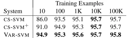
[image:6.595.73.292.63.172.2]CS-SVM+ 91.0 94.9 95.3 95.7 95.7 VAR-SVM 94.9 95.3 95.6 95.7 95.8
Table 2: Accuracy (%) of spell-correction SVMs. Unsupervised accuracy is 94.8%.
examples, while OvA-SVM is better than K-SVM
for small amounts of data.6 K-SVMperforms best
with all the data; it uses the most expressive repre-sentation, but needs 100K examples to make use of it. On the other hand, feature augmentation and variance regularization provide diminishing returns as the amount of training data increases.
4.2 Context-Sensitive Spelling Correction
Context-sensitive spelling correction, or real-word error/malapropism detection (Golding and Roth, 1999; Hirst and Budanitsky, 2005), is the task of identifying errors when a misspelling results in a real word in the lexicon, e.g., using site when sight or cite was intended. Contextual spell checkers are among the most widely-used NLP technology, as they are included in commercial word processing software (Church et al., 2007).
For every occurrence of a word in a pre-defined confusion set (e.g. {cite, sight, cite}), the clas-sifier selects the most likely word from the set. We use the five confusion sets from Bergsma et al. (2009); four are binary and one is a 3-way classi-fication. We use 100K training, 10K development, and 10K test examples for each, and average ac-curacy across the sets. All 2-to-5 gram counts are used in the unsupervised system, so the variance of all weights is regularized in VAR-SVM.
4.2.1 Results
On this task, the majority-class baseline is much higher, 66.9%, and so is the accuracy of the top un-supervised system: 94.8%. Since four of the five sets are binary classifications, where K-SVM and CS-SVMare equivalent, we only give the accuracy of the CS-SVM(it does perform better on the one 3-way set). VAR-SVMagain exceeds the
unsuper-vised accuracy for all training sizes, and generally
6Rifkin and Klautau (2004) argue
Training Examples
System 10 100 1K
CS-SVM 59.0 71.0 84.3
CS-SVM+ 59.4 74.9 84.5
VAR-SVM 70.2 76.2 84.5
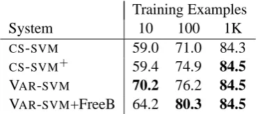
[image:7.595.89.275.62.144.2]VAR-SVM+FreeB 64.2 80.3 84.5
Table 3: Accuracy (%) of non-referential detection SVMs. Unsupervised accuracy is 80.1%.
performs as well as the augmented CS-SVM+ us-ing an order of magnitude less trainus-ing data (Ta-ble 2). Differences from≤1K are significant.
4.3 Non-Referential Pronoun Detection
Non-referential detection predicts whether the En-glish pronoun it refers to a preceding noun (“it lost money”) or is used as a grammatical place-holder (“it is important to...”). This binary clas-sification is a necessary but often neglected step for noun phrase coreference resolution (Paice and Husk, 1987; Bergsma et al., 2008; Ng, 2009).
Bergsma et al. (2008) use features for the counts of various fillers in the pronoun’s context patterns. If it is the most common filler, the pronoun is likely non-referential. If other fillers are common (like they or he), it is likely a referential instance. For example, “he lost money” is common on the web, but “he is important to” is not. We use the same fillers as in previous work, and preprocess the N-gram corpus in the same way.
The unsupervised system picks non-referential if the difference between the summed count of
it fillers and the summed count of they fillers is
above a threshold (note this no longer fits (5), with consequences discussed below). We thus separately minimize the variance of the it pattern weights and the they pattern weights. We use 1K training, 533 development, and 534 test examples.
4.3.1 Results
The most common class is referential, occurring in 59.4% of test examples. The unsupervised sys-tem again does much better, at 80.1%.
Annotated training examples are much harder to obtain for this task and we experiment with a smaller range of training sizes (Table 3). The per-formance of VAR-SVM exceeds the performance of K-SVM across all training sizes (bold accura-cies are significantly better than eitherCS-SVMfor
≤100 examples). However, the gains were not as large as we had hoped, and accuracy remains
worse than the unsupervised system when not us-ing all the trainus-ing data. When usus-ing all the data, a fairly large C-parameter performs best on devel-opment data, so regularization plays less of a role. After development experiments, we speculated that the poor performance relative to the unsuper-vised approach was related to class bias. In the other tasks, the unsupervised system chooses the highest summed score. Here, the difference in it and they counts is compared to a threshold. Since the bias feature is regularized toward zero, then, unlike the other tasks, using a low C-parameter does not produce the unsupervised system, so per-formance can begin below the unsupervised level. Since we wanted the system to learn this thresh-old, even when highly regularized, we removed the regularization penalty from the bias weight, letting the optimization freely set the weight to minimize training error. With more freedom, the new classifier (VAR-SVM+FreeB) performs worse with 10 examples, but exceeds the unsupervised approach with 100 training points. Although this was somewhat successful, developing better strategies for bias remains useful future work.
5 Related Work
There is a large body of work on regularization in machine learning, including work that uses posi-tive semi-definite matrices in the SVM quadratic program. The graph Laplacian has been used to encourage geometrically-similar feature vectors to be classified similarly (Belkin et al., 2006). An ap-pealing property of these approaches is that they incorporate information from unlabeled examples. Wang et al. (2006) use Laplacian regularization for the task of dependency parsing. They regular-ize such that features for distributionally-similar words have similar weights. Rather than penal-ize pairwise differences proportional to a similar-ity function, we simply penalize weight variance.
In the field of computer vision, Tefas et al. (2001) (binary) and Kotsia et al. (2009) (multi-class) also regularize weights with respect to a co-variance matrix. They use labeled data to find the sum of the sample covariance matrices from each class, similar to linear discriminant analysis. We propose the idea in general, and instantiate with a different Cmatrix: a variance regularizer over
¯
w. Most importantly, our instantiated covariance matrix does not require labeled data to generate.
feature correlations in a logistic regression clas-sifier. They propose a method to construct a co-variance matrix for a multivariate Gaussian prior on the classifier’s weights. Labeled data for other, related tasks is used to infer potentially correlated features on the target task. Like in our results, they found that the gains from modeling dependencies diminish as more training data is available.
We also mention two related online learning ap-proaches. Similar to our goal of regularizing to-ward a good unsupervised system, Crammer et al. (2006) regularizew¯toward a (different) target vec-tor at each update, rather than strictly minimizing
||w¯||2
. The target vector is the vector learned from the cumulative effect of previous updates. Dredze et al. (2008) maintain the variance of each weight and use this to guide the online updates. However, covariance between weights is not considered.
We believe new SVM regularizations in gen-eral, and variance regularization in particular, will increasingly be used in combination with related NLP strategies that learn better when labeled data is scarce. These may include: using more-general features, e.g. ones generated from raw text (Miller et al., 2004; Koo et al., 2008), leveraging out-of-domain examples to improve in-out-of-domain classifi-cation (Blitzer et al., 2007; Daum´e III, 2007), ac-tive learning (Cohn et al., 1994; Tong and Koller, 2002), and approaches that treat unlabeled data as labeled, such as bootstrapping (Yarowsky, 1995), co-training (Blum and Mitchell, 1998), and self-training (McClosky et al., 2006).
6 Future Work
The primary direction of future research will be to apply the VAR-SVMto new problems and tasks. There are many situations where a system designer has an intuition about the role a feature will play in prediction; the feature was perhaps added with this role in mind. By biasing the SVM to use features as intended, VAR-SVMmay learn better with fewer training examples. The relationship between at-tributes and classes may be explicit when, e.g., a rule-based system is optimized via discrimina-tive learning, or annotators justify their decisions by indicating the relevant attributes (Zaidan et al., 2007). Also, if features are a priori thought to have different predictive worth, the attribute
val-ues could be scaled such that variance
regulariza-tion, as we formulated it, has the desired effect. Other avenues of future work will be to extend
the VAR-SVM in three directions: efficiency,
rep-resentational power, and problem domain.
While we optimized the VAR-SVMobjective in CPLEX, general purpose QP-solvers “do not ex-ploit the special structure of [the SVM optimiza-tion] problem,” and consequently often train in time super-linear with the number of training ex-amples (Joachims et al., 2009). It would be useful to fit our optimization problem to efficient SVM training methods, especially for linear classifiers.
VAR-SVM’s representational power could be
ex-tended by using non-linear SVMs. Kernels can be used with a covariance regularizer (Kotsia et al., 2009). Since Cis positive semi-definite, the
square root of its inverse is defined. We can there-fore map the input examples using (C−12x¯), and write an equivalent objective function in terms of kernel functions over the transformed examples.
Also, since structured-prediction SVMs build on the multi-class framework (Tsochantaridis et al., 2005), variance regularization can be incor-porated naturally into more complex prediction tasks, such as parsers, taggers, and aligners.
VAR-SVMmay also help in new domains where
annotated data is lacking. VAR-SVM should be
stronger cross-domain than K-SVM; regulariza-tion with domain-neutral prior-knowledge can off-set domain-specific biases. Learned weight vec-tors from other domains may also provide cross-domain regularization guidance.
7 Conclusion
We presented variance-regularization SVMs, an approach to learning that creates better classi-fiers using fewer training examples. Variance reg-ularization incorporates a bias for known good weights into the SVM’s quadratic program. The VAR-SVM can therefore exploit extra knowledge by the system designer. Since the objective re-mains a convex quadratic function of the weights, the program is computationally no harder to opti-mize than a standard SVM. We also demonstrated how to design multi-class SVMs using only class-specific attributes, and compared the performance of this approach to standard multi-class SVMs on the task of preposition selection.
References
Mikhail Belkin, Partha Niyogi, and Vikas Sindhwani. 2006. Manifold regularization: A geometric frame-work for learning from labeled and unlabeled exam-ples. JMLR, 7:2399–2434.
Shane Bergsma, Dekang Lin, and Randy Goebel. 2008. Distributional identification of non-referential pronouns. In ACL-08: HLT.
Shane Bergsma, Dekang Lin, and Randy Goebel. 2009. Web-scale N-gram models for lexical disam-biguation. In IJCAI.
John Blitzer, Mark Dredze, and Fernando Pereira. 2007. Biographies, bollywood, boom-boxes and blenders: Domain adaptation for sentiment classi-fication. In ACL.
Avrim Blum and Tom Mitchell. 1998. Combining la-beled and unlala-beled data with co-training. In COLT.
Thorsten Brants and Alex Franz. 2006. The Google Web 1T 5-gram Corpus Version 1.1. LDC2006T13.
Martin Chodorow, Joel R. Tetreault, and Na-Rae Han. 2007. Detection of grammatical errors involving prepositions. In ACL-SIGSEM Workshop on Prepo-sitions.
Kenneth Church, Ted Hart, and Jianfeng Gao. 2007. Compressing trigram language models with Golomb coding. In EMNLP-CoNLL.
David Cohn, Les Atlas, and Richard Ladner. 1994. Im-proving generalization with active learning. Mach. Learn., 15(2):201–221.
Corinna Cortes and Vladimir Vapnik. 1995. Support-vector networks. Mach. Learn., 20(3):273–297.
CPLEX. 2005. IBM ILOG CPLEX 9.1.www.ilog. com/products/cplex/.
Koby Crammer and Yoram Singer. 2001. On the algo-rithmic implementation of multiclass kernel-based vector machines. JMLR, 2:265–292.
Koby Crammer and Yoram Singer. 2003. Ultracon-servative online algorithms for multiclass problems. JMLR, 3:951–991.
Koby Crammer, Ofer Dekel, Joseph Keshet, Shai Shalev-Shwartz, and Yoram Singer. 2006. Online passive-aggressive algorithms. JMLR, 7:551–585.
Hal Daum´e III. 2007. Frustratingly easy domain adap-tation. In ACL.
Mark Dredze, Koby Crammer, and Fernando Pereira. 2008. Confidence-weighted linear classification. In ICML.
Richard O. Duda and Peter E. Hart. 1973. Pattern Classification and Scene Analysis. John Wiley & Sons.
Rong-En Fan, Kai-Wei Chang, Cho-Jui Hsieh, Xiang-Rui Wang, and Chih-Jen Lin. 2008. LIBLIN-EAR: A library for large linear classification. JMLR, 9:1871–1874.
Andrew R. Golding and Dan Roth. 1999. A Winnow-based approach to context-sensitive spelling correc-tion. Mach. Learn., 34(1-3):107–130.
Sariel Har-Peled, Dan Roth, and Dav Zimak. 2003. Constraint classification for multiclass classification and ranking. In NIPS.
Graeme Hirst and Alexander Budanitsky. 2005. Cor-recting real-word spelling errors by restoring lexical cohesion. Nat. Lang. Eng., 11(1):87–111.
Chih-Wei Hsu and Chih-Jen Lin. 2002. A comparison of methods for multiclass support vector machines. IEEE Trans. Neur. Networks, 13(2):415–425.
Thorsten Joachims, Thomas Finley, and Chun-Nam John Yu. 2009. Cutting-plane training of structural SVMs. Mach. Learn., 77(1):27–59.
Thorsten Joachims. 2002. Optimizing search engines using clickthrough data. In KDD.
Thorsten Joachims. 2006. Training linear SVMs in linear time. In KDD.
Terry Koo, Xavier Carreras, and Michael Collins. 2008. Simple semi-supervised dependency parsing. In ACL-08: HLT.
Irene Kotsia, Stefanos Zafeiriou, and Ioannis Pitas. 2009. Novel multiclass classifiers based on the min-imization of the within-class variance. IEEE Trans. Neur. Networks, 20(1):14–34.
Mirella Lapata and Frank Keller. 2005. Web-based models for natural language processing. ACM Trans. Speech and Language Processing, 2(1):1–31.
David McClosky, Eugene Charniak, and Mark John-son. 2006. Effective self-training for parsing. In HLT-NAACL.
Scott Miller, Jethran Guinness, and Alex Zamanian. 2004. Name tagging with word clusters and discrim-inative training. In HLT-NAACL.
Andrew Y. Ng and Michael I. Jordan. 2002. Discrim-inative vs. generative classifiers: A comparison of logistic regression and naive bayes. In NIPS.
Vincent Ng. 2009. Graph-cut-based anaphoricity de-termination for coreference resolution. In NAACL-HLT.
Franz J. Och and Hermann Ney. 2002. Discriminative training and maximum entropy models for statistical machine translation. In ACL.
Chris D. Paice and Gareth D. Husk. 1987. Towards the automatic recognition of anaphoric features in En-glish text: the impersonal pronoun “it”. Computer Speech and Language, 2:109–132.
Rajat Raina, Andrew Y. Ng, and Daphne Koller. 2006. Constructing informative priors using transfer learn-ing. In ICML.
Ryan Rifkin and Aldebaro Klautau. 2004. In defense of one-vs-all classification. JMLR, 5:101–141.
Noah A. Smith and Jason Eisner. 2005. Contrastive estimation: training log-linear models on unlabeled data. In ACL.
Anastasios Tefas, Constantine Kotropoulos, and Ioan-nis Pitas. 2001. Using support vector machines to enhance the performance of elastic graph matching for frontal face authentication. IEEE Trans. Pattern Anal. Machine Intell., 23:735–746.
Joel R. Tetreault and Martin Chodorow. 2008. The ups and downs of preposition error detection in ESL writing. In COLING.
Simon Tong and Daphne Koller. 2002. Support vec-tor machine active learning with applications to text classification. JMLR, 2:45–66.
Ioannis Tsochantaridis, Thorsten Joachims, Thomas Hofmann, and Yasemin Altun. 2005. Large mar-gin methods for structured and interdependent out-put variables. JMLR, 6:1453–1484.
Vladimir N. Vapnik. 1998. Statistical Learning The-ory. John Wiley & Sons.
Qin Iris Wang, Colin Cherry, Dan Lizotte, and Dale Schuurmans. 2006. Improved large margin depen-dency parsing via local constraints and Laplacian regularization. In CoNLL.
Jason Weston and Chris Watkins. 1998. Multi-class support vector machines. Technical Report CSD-TR-98-04, Department of Computer Science, Royal Holloway, University of London.
David Yarowsky. 1995. Unsupervised word sense dis-ambiguation rivaling supervised methods. In ACL.