Graph Convolutional Encoders
for Syntax-aware Neural Machine Translation
Joost Bastings1 Ivan Titov1,2 Wilker Aziz1
Diego Marcheggiani1 Khalil Sima’an1
1ILLC, University of Amsterdam 2ILCC, University of Edinburgh
{bastings,titov,w.aziz,marcheggiani,k.simaan}@uva.nl
Abstract
We present a simple and effective ap-proach to incorporating syntactic struc-ture into neural attention-based encoder-decoder models for machine translation. We rely on graph-convolutional networks (GCNs), a recent class of neural networks developed for modeling graph-structured data. Our GCNs use predicted syntactic dependency trees of source sentences to produce representations of words (i.e. hid-den states of the encoder) that are sensitive to their syntactic neighborhoods. GCNs take word representations as input and produce word representations as output, so they can easily be incorporated as layers into standard encoders (e.g., on top of bidi-rectional RNNs or convolutional neural networks). We evaluate their effectiveness with English-German and English-Czech translation experiments for different types of encoders and observe substantial im-provements over their syntax-agnostic ver-sions in all the considered setups.
1 Introduction
Neural machine translation (NMT) is one of suc-cess stories of deep learning in natural language processing, with recent NMT systems outperform-ing traditional phrase-based approaches on many language pairs (Sennrich et al.,2016a). State-of-the-art NMT systems rely on sequential encoder-decoders (Sutskever et al.,2014;Bahdanau et al.,
2015) and lack any explicit modeling of syntax or any hierarchical structure of language. One poten-tial reason for why we have not seen much benefit from using syntactic information in NMT is the lack of simple and effective methods for incorpo-rating structured information in neural encoders,
including RNNs. Despite some successes, tech-niques explored so far either incorporate syntactic information in NMT models in a relatively indi-rect way (e.g., multi-task learning (Luong et al.,
2015a;Nadejde et al.,2017;Eriguchi et al.,2017;
Hashimoto and Tsuruoka, 2017)) or may be too restrictive in modeling the interface between syn-tax and the translation task (e.g., learning repre-sentations of linguistic phrases (Eriguchi et al.,
2016)). Our goal is to provide the encoder with access to rich syntactic information but let it de-cide which aspects of syntax are beneficial for MT, without placing rigid constraints on the in-teraction between syntax and the translation task. This goal is in line with claims that rigid syntac-tic constraints typically hurt MT (Zollmann and Venugopal,2006;Smith and Eisner,2006;Chiang,
2010), and, though these claims have been made in the context of traditional MT systems, we believe they are no less valid for NMT.
Attention-based NMT systems (Bahdanau et al.,
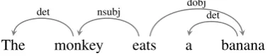
2015;Luong et al., 2015b) represent source stence words as latent-feature vectors in the en-coder and use these vectors when generating a translation. Our goal is to automatically incorpo-rate information about syntactic neighborhoods of source words into these feature vectors, and, thus, potentially improve quality of the translation out-put. Since vectors correspond to words, it is natu-ral for us to use dependency syntax. Dependency trees (see Figure 1) represent syntactic relations between words: for example,monkeyis a subject of the predicateeats, andbananais its object.
In order to produce syntax-aware feature representations of words, we exploit graph-convolutional networks (GCNs) (Duvenaud et al.,
2015;Defferrard et al.,2016;Kearnes et al.,2016;
Kipf and Welling, 2016). GCNs can be regarded as computing a latent-feature representation of a node (i.e. a real-valued vector) based on its k
The monkey eats a banana det nsubj dobjdet
Figure 1: A dependency tree for the example sen-tence: “The monkey eats a banana.”
th order neighborhood (i.e. nodes at mostkhops aways from the node) (Gilmer et al.,2017). They are generally simple and computationally inexpen-sive. We use Syntactic GCNs, a version of GCN operating on top of syntactic dependency trees, re-cently shown effective in the context of semantic role labeling (Marcheggiani and Titov,2017).
Since syntactic GCNs produce representations at word level, it is straightforward to use them as encoders within the attention-based encoder-decoder framework. As NMT systems are trained end-to-end, GCNs end up capturing syntactic properties specifically relevant to the translation task. Though GCNs can take word embeddings as input, we will see that they are more effec-tive when used as layers on top of recurrent neu-ral network (RNN) or convolutional neuneu-ral net-work (CNN) encoders (Gehring et al.,2016), en-riching their states with syntactic information. A comparison to RNNs is the most challenging test for GCNs, as it has been shown that RNNs (e.g., LSTMs) are able to capture certain syntac-tic phenomena (e.g., subject-verb agreement) rea-sonably well on their own, without explicit tree-bank supervision (Linzen et al., 2016;Shi et al.,
2016). Nevertheless, GCNs appear beneficial even in this challenging set-up: we obtain +1.2 and +0.7 BLEU point improvements from using syntactic GCNs on top of bidirectional RNNs for English-German and English-Czech, respectively.
In principle, GCNs are flexible enough to incor-porate any linguistic structure as long as they can be represented as graphs (e.g., dependency-based semantic-role labeling representations (Surdeanu et al., 2008), AMR semantic graphs (Banarescu et al., 2012) and co-reference chains). For ex-ample, unlike recursive neural networks (Socher et al.,2013), GCNs do not require the graphs to be trees. However, in this work we solely focus on dependency syntax and leave more general inves-tigation for future work.
Our main contributions can be summarized as follows:
• we introduce a method for incorporating structure into NMT using syntactic GCNs; • we show that GCNs can be used along with
RNN and CNN encoders;
• we show that incorporating structure is ben-eficial for machine translation on English-Czech and English-German.
2 Background
Notation. We use x for vectors, x1:t for a se-quence oftvectors, andXfor matrices. Thei-th value of vectorxis denoted by xi. We use◦for vector concatenation.
2.1 Neural Machine Translation
In NMT (Kalchbrenner and Blunsom, 2013;
Sutskever et al., 2014; Cho et al., 2014b), given example translation pairs from a parallel corpus, a neural network is trained to directly estimate the conditional distributionp(y1:Ty|x1:Tx)of translat-ing a source sentence x1:Tx (a sequence of Tx words) into a target sentence y1:Ty. NMT mod-els typically consist of an encoder, a decoder and some method for conditioning the decoder on the encoder, for example, an attention mechanism. We will now briefly describe the components that we use in this paper.
2.1.1 Encoders
An encoder is a function that takes as input the source sentence and produces a representation en-coding its semantic content. We describe recur-rent, convolutional and bag-of-words encoders. Recurrent. Recurrent neural networks (RNNs) (Elman, 1990) model sequential data. They re-ceive one input vector at each time step and up-date their hidden state to summarize all inputs up to that point. Given an input sequence x1:Tx =
x1,x2, . . . ,xTx of word embeddings an RNN is defined recursively as follows:
RNN(x1:t) =f(xt,RNN(x1:t−1)) wheref is a nonlinear function such as an LSTM (Hochreiter and Schmidhuber, 1997) or a GRU (Cho et al.,2014b). We will use the function RNN as an abstract mapping from an input sequence
Cardie,2014) is often used. A bidirectional RNN reads the input sentence in two directions and then concatenates the states for each time step:
BIRNN(x1:Tx, t) =RNNF(x1:t)◦RNNB(xTx:t)
where RNNF and RNNB are the forward and backward RNNs, respectively. For further details we refer to the encoder ofBahdanau et al.(2015). Convolutional. Convolutional Neural Networks (CNNs) apply a fixed-size window over the input sequence to capture the local context of each word (Gehring et al.,2016). One advantage of this ap-proach over RNNs is that it allows for fast parallel computation, while sacrificing non-local context. To remedy the loss of context, multiple CNN lay-ers can be stacked. Formally, given an input se-quencex1:Tx, we define a CNN as follows:
CNN(x1:Tx, t) =f(xt−bw/2c, ..,xt, ..,xt+bw/2c)
where f is a nonlinear function, typically a lin-ear transformation followed by ReLU, andwis the size of the window.
Bag-of-Words. In a bag-of-words (BoW) en-coder every word is simply represented by its word embedding. To give the decoder some sense of word position, position embeddings (PE) may be added. There are different strategies for defining position embeddings, and in this paper we choose to learn a vector for each absolute word position up to a certain maximum length. We then repre-sent thet-th word in a sequence as follows:
BOW(x1:Tx, t) =xt+pt
wherextis the word embedding andptis the t-th position embedding.
2.1.2 Decoder
A decoder produces the target sentence condi-tioned on the representation of the source sentence induced by the encoder. InBahdanau et al.(2015) the decoder is implemented as an RNN condi-tioned on an additional inputci, the context vector, which is dynamically computed at each time step using an attention mechanism.
The probability of a target word yi is now a function of the decoder RNN state, the previous target word embedding, and the context vector. The model is trained end-to-end for maximum log likelihood of the next target word given its context.
2.2 Graph Convolutional Networks
We will now describe the Graph Convolutional Networks (GCNs) of Kipf and Welling (2016). For a comprehensive overview of alternative GCN architectures seeGilmer et al.(2017).
A GCN is a multilayer neural network that operates directly on a graph, encoding informa-tion about the neighborhood of a node as a real-valued vector. In each GCN layer, information flows along edges of the graph; in other words, each node receives messages from all its imme-diate neighbors. When multiple GCN layers are stacked, information about larger neighborhoods gets integrated. For example, in the second layer, a node will receive information from its immediate neighbors, but this information already includes information from their respective neighbors. By choosing the number of GCN layers, we regulate the distance the information travels: with k lay-ers a node receives information from neighbors at mostkhops away.
Formally, consider an undirected graph G = (V,E), where V is a set of n nodes, and E is a set of edges. Every node is assumed to be con-nected to itself, i.e. ∀v ∈ V : (v, v) ∈ E.Now, letX ∈Rd×nbe a matrix containing allnnodes with their features, wheredis the dimensionality of the feature vectors. In our case,Xwill contain word embeddings, but in general it can contain any kind of features. For a 1-layer GCN, the new node representations are computed as follows:
hv =ρ
X
u∈N(v)
Wxu+b
!
whereW ∈Rd×dis a weight matrix andb ∈Rd a bias vector.1 ρis an activation function, e.g. a
ReLU.N(v)is the set of neighbors ofv, which we assume here to always includevitself. As stated before, to allow information to flow over multiple hops, we need to stack GCN layers. The recursive computation is as follows:
h(vj+1) =ρ X
u∈N(v)
W(j)h(uj)+b(j)
!
wherejindexes the layer, andh(0)v =xv.
1We dropped the normalization factor used by Kipf
and Welling (2016), as it is not used in syntactic GCNs
W(0)det W(0)nsubj
W(0)
dobj
W(0)det
W(1)det W(1)nsubj
W(1)
dobj
W(1)det
*PAD* The monkey eats a banana *PAD*
h(0)
h(1)
h(2)
GCN
[image:4.595.83.505.68.251.2]CNN
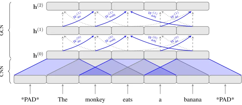
Figure 2: A 2-layer syntactic GCN on top of a convolutional encoder. Loop connections are depicted with dashed edges, syntactic ones with solid (dependents to heads) and dotted (heads to dependents) edges. Gates and some labels are omitted for clarity.
2.3 Syntactic GCNs
Marcheggiani and Titov(2017) generalize GCNs to operate on directed and labeled graphs.2 This
makes it possible to use linguistic structures such as dependency trees, where directionality and edge labels play an important role. They also integrate edge-wise gates which let the model regulate con-tributions of individual dependency edges. We will briefly describe these modifications.
Directionality. In order to deal with direction-ality of edges, separate weight matrices are used for incoming and outgoing edges. We follow the convention that in dependency trees heads point to their dependents, and thusoutgoing edges are used for head-to-dependent connections, and in-comingedges are used for dependent-to-head con-nections. Modifying the recursive computation for directionality, we arrive at:
h(vj+1)=ρ X
u∈N(v)
Wdir((j)u,v)hu(j)+b(dir(j)u,v)
!
where dir(u, v) selects the weight matrix associ-ated with the directionality of the edge connecting u andv (i.e. WIN for u-to-v, WOUT for v-to-u, and WLOOP for v-to-v). Note that self loops are modeled separately,
so there are now three times as many parameters as in a non-directional GCN.
2For an alternative approach to integrating labels and
di-rections, see applications of GCNs to statistical relation learn-ing (Schlichtkrull et al.,2017).
Labels. Making the GCN sensitive to labels is straightforward given the above modifications for directionality. Instead of using separate matrices for each direction, separate matrices are now de-fined for each direction and label combination:
h(j+1) v =ρ
X
u∈N(v)
Wlab((j)u,v)h(j)
u +b(lab(j) u,v)
!
where we incorporate the directionality of an edge directly in its label.
Importantly, to prevent over-parametrization, only bias terms are made label-specific, in other words: Wlab(u,v) = Wdir(u,v). The resulting syn-tactic GCN is illustrated in Figure2(shown on top of a CNN, as we will explain in the subsequent section).
Edge-wise gating. Syntactic GCNs also include gates, which can down-weight the contribution of individual edges. They also allow the model to deal with noisy predicted structure, i.e. to ignore potentially erroneous syntactic edges. For each edge, a scalar gate is calculated as follows:
g(u,vj) =σh(uj)·wˆ(dir(j)u,v)+ ˆb(lab(j) u,v)
where σ is the logistic sigmoid function, and
ˆ
w(dir(j)u,v) ∈ Rd andˆb(j)
lab(u,v) ∈ Rare learned pa-rameters for the gate. The computation becomes:
h(vj+1)=ρ X
u∈N(v)
3 Graph Convolutional Encoders
In this work we focus on exploiting structural in-formation on the source side, i.e. in the encoder. We hypothesize that using an encoder that incor-porates syntax will lead to more informative rep-resentations of words, and that these representa-tions, when used as context vectors by the decoder, will lead to an improvement in translation qual-ity. Consequently, in all our models, we use the decoder of Bahdanau et al. (2015) and keep this part of the model constant. As is now common practice, we do not use a maxout layer in the de-coder, but apart from this we do not deviate from the original definition. In all models we make use of GRUs (Cho et al.,2014b) as our RNN units.
Our models vary in the encoder part, where we exploit the power of GCNs to induce syntactically-aware representations. We now define a series of encoders of increasing complexity.
BoW + GCN. In our first and simplest model, we propose a bag-of-words encoder (with position embeddings, see§2.1.1), with a GCN on top. In other words, inputsh(0) are a sum of embeddings of a word and its position in a sentence. Since the original BoW encoder captures the linear order-ing information only in a very crude way (through the position embeddings), the structural informa-tion provided by GCN should be highly beneficial.
Convolutional + GCN. In our second model, we use convolutional neural networks to learn word representations. CNNs are fast, but by def-inition only use a limited window of context. In-stead of the approach used byGehring et al.(2016) (i.e. stacking mulitple CNN layers on top of each other), we use a GCN to enrich the one-layer CNN representations. Figure2shows this model. Note that, while the figure shows a CNN with a window size of 3, we will use a larger window size of 5 in our experiments. We expect this model to perform better than BoW + GCN, because of the additional local context captured by the CNN.
BiRNN + GCN. In our third and most powerful model, we employ bidirectional recurrent neural networks. In this model, we start by encoding the source sentence using a BiRNN (i.e. BiGRU), and use the resulting hidden states as input to a GCN. Instead of relying on linear order only, the GCN will allow the encoder to ‘teleport’ over parts of the input sentence, along dependency edges,
con-necting words that otherwise might be far apart. The model might not only benefit from this tele-porting capability however; also the nature of the relations between words (i.e. dependency relation types) may be useful, and the GCN exploits this information (see§2.3for details).
This is the most challenging setup for GCNs, as RNNs have been shown capable of capturing at least some degree of syntactic information with-out explicit supervision (Linzen et al.,2016), and hence they should be hard to improve on by incor-porating treebank syntax.
Marcheggiani and Titov(2017) did not observe improvements from using multiple GCN layers in semantic role labeling. However, we do expect that propagating information from further in the tree should be beneficial in principle. We hypoth-esize that the first layer is the most influential one, capturing most of the syntactic context, and that additional layers only modestly modify the repre-sentations. To ease optimization, we add a resid-ual connection (He et al.,2016) between the GCN layers, when using more than one layer.
4 Experiments
Experiments are performed using the Neural Mon-key toolkit3 (Helcl and Libovick´y, 2017), which
implements the model of Bahdanau et al. (2015) in TensorFlow. We use the Adam optimizer (Kingma and Ba, 2015) with a learning rate of 0.001 (0.0002 for CNN models).4 The batch size
is set to 80. Between layers we apply dropout with a probability of 0.2, and in experiments with GCNs5 we use the same value for edge dropout.
We train for 45 epochs, evaluating the BLEU per-formance of the model every epoch on the vali-dation set. For testing, we select the model with the highest validation BLEU. L2 regularization is used with a value of10−8. All the model selection (incl. hyperparameter selections) was performed on the validation set. In all experiments we obtain translations using a greedy decoder, i.e. we se-lect the output token with the highest probability at each time step.
We will describe an artificial experiment in§4.1
and MT experiments in§4.2.
3https://github.com/ufal/neuralmonkey
4LikeGehring et al.(2016) we note that Adam is too
ag-gressive for CNN models, hence we use a lower learning rate.
4.1 Reordering artificial sequences
Our goal here is to provide an intuition for the ca-pabilities of GCNs. We define a reordering task where randomly permuted sequences need to be put back into the original order. We encode the original order using edges, and test if GCNs can successfully exploit them. Note that this task is not meant to provide a fair comparison to RNNs. The input (besides the edges) simply does not carry any information about the original ordering, so RNNs cannot possibly solve this task.
Data. From a vocabulary of 26 types, we gen-erate random sequences of 3-10 tokens. We then randomly permute them, pointing every token to its original predecessor with a label sampled from a set of 5 labels. Additionally, we point every to-ken to anarbitraryposition in the sequence with a label from a distinct set of 5 ‘fake’ labels. We sam-ple 25000 training and 1000 validation sequences. Model. We use the BiRNN + GCN model, i.e. a bidirectional GRU with a 1-layer GCN on top. We use 32, 64 and 128 units for embeddings, GRU units and GCN layers, respectively.
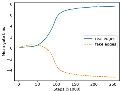
Results. After 6 epochs of training, the model learns to put permuted sequences back into or-der, reaching a validation BLEU of 99.2. Fig-ure 3 shows that the mean values of the bias terms of gates (i.e. ˆb) for real and fake edges are far apart, suggesting that the GCN learns to dis-tinguish them. Interestingly, this illustrates why edge-wise gating is beneficial. A gate-less model would not understand which of the two outgoing arcs is fake and which is genuine, because only biases b would then be label-dependent. Conse-quently, it would only do a mediocre job in re-ordering. Although using label-specific matrices W would also help, this would not scale to the real scenario (see§2.3).
4.2 Machine Translation
Data. For our experiments we use the En-De and En-Cs News Commentary v11 data from the WMT16 translation task.6 For En-De we also
train on the full WMT16 data set. As our valida-tion set and test set we usenewstest2015and
newstest2016, respectively.
Pre-processing. The English sides of the cor-pora are tokenized and parsed into dependency
6http://www.statmt.org/wmt16/translation-task.html
0 50 100 150 200 250
Steps (x1000) 4
2 0 2 4 6 8
Mean gate bias
[image:6.595.309.514.59.215.2]real edges fake edges
Figure 3: Mean values of gate bias terms for real (useful) labels and for fake (non useful) labels sug-gest the GCN learns to distinguish them.
trees by SyntaxNet,7 using the pre-trained Parsey
McParseface model.8 The Czech and German
sides are tokenized using the Moses tokenizer.9
Sentence pairs where either side is longer than 50 words are filtered out after tokenization.
Vocabularies. For the English sides, we con-struct vocabularies from all words except those with a training set frequency smaller than three. For Czech and German, to deal with rare words and phenomena such as inflection and compound-ing, we learn byte-pair encodings (BPE) as de-scribed bySennrich et al.(2016b). Given the size of our data set, and followingWu et al.(2016), we use 8000 BPE merges to obtain robust frequencies for our subword units (16000 merges for full data experiment). Data set statistics are summarized in Table1and vocabulary sizes in Table2.
Train Val. Test
English-German 226822 2169 2999
English-German (full) 4500966 2169 2999
English-Czech 181112 2656 2999
Table 1: The number of sentences in our data sets.
Hyperparameters. We use 256 units for word embeddings, 512 units for GRUs (800 for En-De full data set experiment), and 512 units for con-volutional layers (or equivalently, 512 ‘channels’). The dimensionality of the GCN layers is
equiva-7https://github.com/tensorflow/models/tree/master/syntaxnet 8The used dependency parses can be reproduced by using
thesyntaxnet/demo.shshell script.
[image:6.595.309.523.540.606.2]Source Target
English-German 37824 8099 (BPE)
English-German (full) 50000 16000 (BPE)
English-Czech 33786 8116 (BPE)
Table 2: Vocabulary sizes.
lent to the dimensionality of their input. We report results for 2-layer GCNs, as we find them most ef-fective (see ablation studies below).
Baselines. We provide three baselines, each with a different encoder: a bag-of-words encoder, a convolutional encoder with window sizew= 5, and a BiRNN. See§2.1.1for details.
Evaluation. We report (cased) BLEU results (Papineni et al., 2002) using multi-bleu, as well as Kendallτ reordering scores.10
4.2.1 Results
English-German. Table 3 shows test results on English-German. Unsurprisingly, the bag-of-words baseline performs the worst. We expected the BoW+GCN model to make easy gains over this baseline, which is indeed what happens. The CNN baseline reaches a higher BLEU4 score than the BoW models, but interestingly its BLEU1 score is lower than the BoW+GCN model. The CNN+GCN model improves over the CNN base-line by +1.9 and +1.1 for BLEU1and BLEU4, re-spectively. The BiRNN, the strongest baseline, reaches a BLEU4 of 14.9. Interestingly, GCNs still manage to improve the result by +2.3 BLEU1 and +1.2 BLEU4points. Finally, we observe a big jump in BLEU4by using the full data set and beam search (beam 12). The BiRNN now reaches 23.3, while adding a GCN achieves a score of 23.9. English-Czech. Table 4 shows test results on English-Czech. While it is difficult to obtain high absolute BLEU scores on this dataset, we can still see similar relative improvements. Again the BoW baseline scores worst, with the BoW+GCN eas-ily beating that result. The CNN baseline scores BLEU4 of 8.1, but the CNN+GCN improves on that, this time by +1.0 and +0.6 for BLEU1 and BLEU4, respectively. Interestingly, BLEU1scores for the BoW+GCN and CNN+GCN models are
10SeeStanojevi´c and Simaan(2015). TER (Snover et al.,
2006) and BEER (Stanojevi´c and Sima’an, 2014) metrics, even though omitted due to space considerations, are con-sistent with the reported results.
Kendall BLEU1 BLEU4
BoW 0.3352 40.6 9.5
+ GCN 0.3520 44.9 12.2
CNN 0.3601 42.8 12.6
+ GCN 0.3777 44.7 13.7
BiRNN 0.3984 45.2 14.9
+ GCN 0.4089 47.5 16.1
BiRNN (full) 0.5440 53.0 23.3
[image:7.595.318.514.65.213.2]+ GCN 0.5555 54.6 23.9
Table 3: Test results for English-German.
higher than both baselines so far. Finally, the BiRNN baseline scores a BLEU4 of 8.9, but it is again beaten by the BiRNN+GCN model with +1.9 BLEU1 and +0.7 BLEU4.
Kendall BLEU1 BLEU4
BoW 0.2498 32.9 6.0
+ GCN 0.2561 35.4 7.5
CNN 0.2756 35.1 8.1
+ GCN 0.2850 36.1 8.7
BiRNN 0.2961 36.9 8.9
[image:7.595.325.507.323.436.2]+ GCN 0.3046 38.8 9.6
Table 4: Test results for English-Czech.
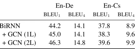
Effect of GCN layers. How many GCN layers do we need? Every layer gives us an extra hop in the graph and expands the syntactic neighbor-hood of a word. Table5shows validation BLEU performance as a function of the number of GCN layers. For English-German, using a 1-layer GCN improves BLEU-1, but surprisingly has little effect on BLEU4. Adding an additional layer gives im-provements on both BLEU1 and BLEU4 of +1.3 and +0.73, respectively. For English-Czech, per-formance increases with each added GCN layer.
En-De En-Cs
BLEU1 BLEU4 BLEU1 BLEU4
BiRNN 44.2 14.1 37.8 8.9
+ GCN (1L) 45.0 14.1 38.3 9.6
[image:7.595.309.525.638.717.2]+ GCN (2L) 46.3 14.8 39.6 9.9
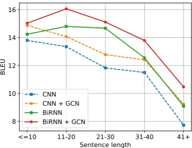
Effect of sentence length. We hypothesize that GCNs should be more beneficial for longer sen-tences: these are likely to contain long-distance syntactic dependencies which may not be ade-quately captured by RNNs but directly encoded in GCNs. To test this, we partition the validation data into five buckets and calculate BLEU for each of them. Figure4shows that GCN-based models outperform their respective baselines rather uni-formly across all buckets. This is a surprising re-sult. One explanation may be that syntactic parses are noisier for longer sentences, and this prevents us from obtaining extra improvements with GCNs.
<=10 11-20 21-30 31-40 41+
Sentence length 8
10 12 14 16
BLEU
[image:8.595.78.271.248.397.2]CNN CNN + GCN BiRNN BiRNN + GCN
Figure 4: Validation BLEU per sentence length.
Discussion. Results suggest that the syntax-aware representations provided by GCNs consis-tently lead to improved translation performance as measured by BLEU4 (as well as TER and BEER). Consistent gains in terms of Kendall tau and BLEU1 indicate that improvements correlate with better word order and lexical/BPE selection, two phenomena that depend crucially on syntax. 5 Related Work
We review various accounts to syntax in NMT as well as other convolutional encoders.
Syntactic features and/or constraints. Sen-nrich and Haddow(2016) embed features such as POS-tags, lemmas and dependency labels and feed these into the network along with word embed-dings. Eriguchi et al. (2016) parse English sen-tences with an HPSG parser and use a Tree-LSTM to encode the internal nodes of the tree. In the decoder, word and node representations compete under the same attention mechanism. Stahlberg et al.(2016) use a pruned lattice from a hierarchi-cal phrase-based model (hiero) to constrain NMT.
Hiero trees are not syntactically-aware, but instead constrained by symmetrized word alignments.
Aharoni and Goldberg (2017) propose neural string-to-tree by predicting linearized parse trees.
Multi-task Learning. Sharing NMT parameters with a syntactic parser is a popular approach to obtaining syntactically-aware representations. Lu-ong et al.(2015a) predict linearized constituency parses as an additional task.Eriguchi et al.(2017) multi-task with a target-side RNNG parser (Dyer et al., 2016) and improve on various language pairs with English on the target side.Nadejde et al.
(2017) multi-task with CCG tagging, and also in-tegrate syntax on the target side by predicting a se-quence of words interleaved with CCG supertags.
Latent structure. Hashimoto and Tsuruoka
(2017) add a syntax-inspired encoder on top of a BiLSTM layer. They encode source words as a learned average of potential parents emulating a relaxed dependency tree. While their model is trained purely on translation data, they also ex-periment with pre-training the encoder using tree-bank annotation and report modest improvements on English-Japanese. Yogatama et al.(2016) in-troduce a model for language understanding and generation that composes words into sentences by inducing unlabeled binary bracketing trees.
Convolutional encoders. Gehring et al. (2016) show that CNNs can be competitive to BiRNNs when used as encoders. To increase the receptive field of a word’s context they stack multiple CNN layers.Kalchbrenner et al.(2016) use convolution in both the encoder and the decoder; they make use of dilation to increase the receptive field. In con-trast to both approaches, we use a GCN informed by dependency structure to increase it. Finally,
Cho et al. (2014a) propose a recursive convolu-tional neural network which builds a tree out of the word leaf nodes, but which ends up compress-ing the source sentence in a scompress-ingle vector.
6 Conclusions
be-yond syntax, by using semantic annotations such as SRL and AMR, and co-reference chains.
Acknowledgments
We would like to thank Michael Schlichtkrull and Thomas Kipf for their suggestions and comments. This work was supported by the European Re-search Council (ERC StG BroadSem 678254) and the Dutch National Science Foundation (NWO VIDI 639.022.518, NWO VICI 277-89-002).
References
Roee Aharoni and Yoav Goldberg. 2017. Towards String-to-Tree Neural Machine Translation. ArXiv e-prints.
Dzmitry Bahdanau, Kyunghyun Cho, and Yoshua Ben-gio. 2015. Neural Machine Translation by Jointly Learning to Align and Translate. InProceedings of the International Conference on Learning Represen-tations (ICLR).
Laura Banarescu, Claire Bonial, Shu Cai, Madalina Georgescu, Kira Griffitt, Ulf Hermjakob, Kevin Knight, Philipp Koehn, Martha Palmer, and Nathan Schneider. 2012. Abstract meaning representation (amr) 1.0 specification. In Conference on Empiri-cal Methods in Natural Language Processing, pages 1533–1544.
David Chiang. 2010. Learning to translate with source and target syntax. InProceedings of the 48th Annual Meeting of the Association for Computational Lin-guistics, pages 1443–1452, Uppsala, Sweden. Asso-ciation for Computational Linguistics.
KyungHyun Cho, Bart van Merrienboer, Dzmitry Bah-danau, and Yoshua Bengio. 2014a. On the Prop-erties of Neural Machine Translation: Encoder-Decoder Approaches. InSSST-8, Eighth Workshop on Syntax, Semantics and Structure in Statistical Translation, volume abs/1409.1259, pages 103–111. Kyunghyun Cho, Bart van Merrienboer, Caglar Gul-cehre, Dzmitry Bahdanau, Fethi Bougares, Hol-ger Schwenk, and Yoshua Bengio. 2014b. Learn-ing Phrase Representations usLearn-ing RNN Encoder– Decoder for Statistical Machine Translation. In Pro-ceedings of the 2014 Conference on Empirical Meth-ods in Natural Language Processing (EMNLP), pages 1724–1734, Doha, Qatar. Association for Computational Linguistics.
Micha¨el Defferrard, Xavier Bresson, and Pierre Van-dergheynst. 2016. Convolutional neural networks on graphs with fast localized spectral filtering. In
Advances in Neural Information Processing Sys-tems 29: Annual Conference on Neural Information Processing Systems 2016, December 5-10, 2016, Barcelona, Spain, pages 3837–3845.
David K Duvenaud, Dougal Maclaurin, Jorge Ipar-raguirre, Rafael Bombarell, Timothy Hirzel, Al´an Aspuru-Guzik, and Ryan P Adams. 2015. Convo-lutional networks on graphs for learning molecular fingerprints. InAdvances in neural information pro-cessing systems, pages 2224–2232.
Chris Dyer, Adhiguna Kuncoro, Miguel Ballesteros, and Noah A. Smith. 2016. Recurrent neural network grammars. InProceedings of the 2016 Conference of the North American Chapter of the Association for Computational Linguistics: Human Language Technologies, pages 199–209, San Diego, Califor-nia. Association for Computational Linguistics.
Jeffrey L Elman. 1990. Finding structure in time. Cog-nitive science, 14(2):179–211.
Akiko Eriguchi, Kazuma Hashimoto, and Yoshimasa Tsuruoka. 2016. Tree-to-sequence attentional neu-ral machine translation. InProceedings of the 54th Annual Meeting of the Association for Computa-tional Linguistics (Volume 1: Long Papers), pages 823–833, Berlin, Germany. Association for Compu-tational Linguistics.
Akiko Eriguchi, Yoshimasa Tsuruoka, and Kyunghyun Cho. 2017. Learning to Parse and Translate Im-proves Neural Machine Translation.ArXiv e-prints. Jonas Gehring, Michael Auli, David Grangier, and Yann N. Dauphin. 2016. A convolutional en-coder model for neural machine translation. CoRR, abs/1611.02344.
Justin Gilmer, Samuel S. Schoenholz, Patrick F. Riley, Oriol Vinyals, and George E. Dahl. 2017. Neural Message Passing for Quantum Chemistry. ArXiv e-prints.
Kazuma Hashimoto and Yoshimasa Tsuruoka. 2017.
Neural machine translation with source-side latent graph parsing.CoRR, abs/1702.02265.
Kaiming He, Xiangyu Zhang, Shaoqing Ren, and Jian Sun. 2016. Deep residual learning for image recog-nition. InProceedings of the IEEE Conference on Computer Vision and Pattern Recognition, pages 770–778.
Jindˇrich Helcl and Jindˇrich Libovick´y. 2017. Neural monkey: An open-source tool for sequence learn-ing. The Prague Bulletin of Mathematical Linguis-tics, (107):5–17.
Sepp Hochreiter and J¨urgen Schmidhuber. 1997.
Long Short-Term Memory. Neural Computation, 9(8):1735–1780.
Nal Kalchbrenner and Phil Blunsom. 2013. Recurrent Continuous Translation Models. InProceedings of the 2013 Conference on Empirical Methods in Natu-ral Language Processing, pages 1700–1709, Seattle, Washington, USA.
Nal Kalchbrenner, Lasse Espeholt, Karen Simonyan, A¨aron van den Oord, Alex Graves, and Koray Kavukcuoglu. 2016. Neural machine translation in linear time.CoRR, abs/1610.10099.
Steven Kearnes, Kevin McCloskey, Marc Berndl, Vijay Pande, and Patrick Riley. 2016. Molecular graph convolutions: moving beyond fingerprints. Jour-nal of computer-aided molecular design, 30(8):595– 608.
Diederik P. Kingma and Jimmy Ba. 2015. Adam: A method for stochastic optimization. InICLR. Thomas N. Kipf and Max Welling. 2016.
Semi-supervised classification with graph convolutional networks.CoRR, abs/1609.02907.
Tal Linzen, Emmanuel Dupoux, and Yoav Goldberg. 2016.Assessing the ability of lstms to learn syntax-sensitive dependencies. Transactions of the Associ-ation for ComputAssoci-ational Linguistics, 4:521–535. Minh-Thang Luong, Quoc V. Le, Ilya Sutskever,
Oriol Vinyals, and Lukasz Kaiser. 2015a. Multi-task Sequence to Sequence Learning. CoRR, abs/1511.06114.
Thang Luong, Hieu Pham, and Christopher D. Man-ning. 2015b. Effective Approaches to Attention-based Neural Machine Translation. In Proceed-ings of the 2015 Conference on Empirical Meth-ods in Natural Language Processing, pages 1412– 1421, Lisbon, Portugal. Association for Computa-tional Linguistics.
Diego Marcheggiani and Ivan Titov. 2017. Encoding Sentences with Graph Convolutional Networks for Semantic Role Labeling. InProceedings of the 2017 Conference on Empirical Methods in Natural Lan-guage Processing, Copenhagen, Denmark. Associa-tion for ComputaAssocia-tional Linguistics.
Maria Nadejde, Siva Reddy, Rico Sennrich, Tomasz Dwojak, Marcin Junczys-Dowmunt, Philipp Koehn, and Alexandra Birch. 2017. Syntax-aware Neural Machine Translation Using CCG.ArXiv e-prints. Kishore Papineni, Salim Roukos, Todd Ward, and Wei
jing Zhu. 2002. Bleu: a method for automatic eval-uation of machine translation. pages 311–318. Michael Schlichtkrull, Thomas N Kipf, Peter Bloem,
Rianne van den Berg, Ivan Titov, and Max Welling. 2017.Modeling Relational Data with Graph Convo-lutional Networks.ArXiv e-prints.
Mike Schuster and Kuldip K. Paliwal. 1997. Bidirec-tional recurrent neural networks.IEEE Transactions on Signal Processing, 45(11):2673–2681.
Rico Sennrich and Barry Haddow. 2016.Linguistic In-put Features Improve Neural Machine Translation. InProceedings of the First Conference on Machine Translation (WMT16), volume abs/1606.02892.
Rico Sennrich, Barry Haddow, and Alexandra Birch. 2016a. Edinburgh neural machine translation sys-tems for wmt 16. In Proceedings of the First Conference on Machine Translation, pages 371– 376, Berlin, Germany. Association for Computa-tional Linguistics.
Rico Sennrich, Barry Haddow, and Alexandra Birch. 2016b. Neural machine translation of rare words with subword units. InProceedings of the 54th An-nual Meeting of the Association for Computational Linguistics (Volume 1: Long Papers), pages 1715– 1725, Berlin, Germany. Association for Computa-tional Linguistics.
Xing Shi, Inkit Padhi, and Kevin Knight. 2016. Does string-based neural mt learn source syntax? In Pro-ceedings of the 2016 Conference on Empirical Meth-ods in Natural Language Processing, pages 1526– 1534, Austin, Texas. Association for Computational Linguistics.
David Smith and Jason Eisner. 2006. Quasi-synchronous grammars: Alignment by soft projec-tion of syntactic dependencies. In Proceedings on the Workshop on Statistical Machine Translation, pages 23–30, New York City. Association for Com-putational Linguistics.
Matthew Snover, Bonnie Dorr, Richard Schwartz, Lin-nea Micciulla, and John Makhoul. 2006. A study of translation edit rate with targeted human annota-tion. InIn Proceedings of Association for Machine Translation in the Americas, pages 223–231.
Richard Socher, Alex Perelygin, Jean Wu, Jason Chuang, Christopher D. Manning, Andrew Ng, and Christopher Potts. 2013. Recursive deep models for semantic compositionality over a sentiment tree-bank. InProceedings of EMNLP.
Felix Stahlberg, Eva Hasler, Aurelien Waite, and Bill Byrne. 2016. Syntactically guided neural machine translation. InProceedings of the 54th Annual Meet-ing of the Association for Computational LMeet-inguistics (Volume 2: Short Papers), pages 299–305, Berlin, Germany. Association for Computational Linguis-tics.
Miloˇs Stanojevi´c and Khalil Simaan. 2015. Evaluating mt systems with beer. The Prague Bulletin of Math-ematical Linguistics, 104(1):17–26.
Mihai Surdeanu, Richard Johansson, Adam Meyers, Llu´ıs M`arquez, and Joakim Nivre. 2008. The conll 2008 shared task on joint parsing of syntactic and semantic dependencies. InProceedings of CoNLL. Ilya Sutskever, Oriol Vinyals, and Quoc V. Le. 2014.
Sequence to Sequence Learning with Neural Net-works. InNeural Information Processing Systems (NIPS), pages 3104–3112.
Yonghui Wu, Mike Schuster, Zhifeng Chen, Quoc V. Le, Mohammad Norouzi, Wolfgang Macherey, Maxim Krikun, Yuan Cao, Qin Gao, Klaus Macherey, Jeff Klingner, Apurva Shah, Melvin Johnson, Xiaobing Liu, Lukasz Kaiser, Stephan Gouws, Yoshikiyo Kato, Taku Kudo, Hideto Kazawa, Keith Stevens, George Kurian, Nishant Patil, Wei Wang, Cliff Young, Jason Smith, Jason Riesa, Alex Rudnick, Oriol Vinyals, Greg Corrado, Macduff Hughes, and Jeffrey Dean. 2016. Google’s neural machine translation system: Bridging the gap between human and machine translation. CoRR, abs/1609.08144.
Dani Yogatama, Phil Blunsom, Chris Dyer, Edward Grefenstette, and Wang Ling. 2016. Learning to compose words into sentences with reinforcement learning.CoRR, abs/1611.09100.