Refining Generative Language Models using Discriminative Learning
Ben Sandbank
Blavatnik School of Computer Science Tel-Aviv University
Tel-Aviv 69978, Israel [email protected]
Abstract
We propose a new approach to language mod-eling which utilizes discriminative learning methods. Our approach is an iterative one: starting with an initial language model, in each iteration we generate 'false' sentences from the current model, and then train a clas-sifier to discriminate between them and sen-tences from the training corpus. To the extent that this succeeds, the classifier is incorpo-rated into the model by lowering the probabil-ity of sentences classified as false, and the process is repeated. We demonstrate the effec-tiveness of this approach on a natural lan-guage corpus and show it provides an 11.4% improvement in perplexity over a modified kneser-ney smoothed trigram.
1 Introduction
Language modeling is a fundamental task in natu-ral language processing and is routinely employed in a wide range of applications, such as speech recognition, machine translation, etc’. Tradition-ally, a language model is a probabilistic model which assigns a probability value to a sentence or a sequence of words. We refer to these as generative language models. A very popular example of a generative language model is the n-gram, which conditions the probability of the next word on the previous (n-1)-words.
Although simple and widely-applicable, it has proven difficult to allow n-grams, and other forms of generative language models as well, to take
ad-vantage of non-local and overlapping features.1 These sorts of features, however, pose no problem for standard discriminative learning methods, e.g. large-margin classifiers. For this reason, a new class of language model, the discriminative lan-guage model, has been proposed recently to aug-ment generative language models (Gao et al., 2005; Roark et al., 2007). Instead of providing probability values, discriminative language models directly classify sentences as either correct or in-correct, where the definition of correctness de-pends on the application (e.g. grammatical / ungrammatical, correct translation / incorrect trans-lation, etc').
Discriminative learning methods require negative samples. Given that the corpora used for training language models contain only real sentences, i.e. positive samples, obtaining these can be problematic. In most work on discriminative language modeling this was not a major issue as the work was concerned with specific applications, and these provided a natural definition of negative samples. For instance, (Roark et al., 2007) proposed a discriminative language model for a speech recognition task. Given an acoustic sequence, a baseline recognizer was used to generate a set of possible transcriptions. The correct transcription was taken as a positive sample, while the rest were taken as negative samples. More recently, however, Okanohara and Tsujii (2007) showed that a
1
Conditional maximum entropy models (Rosenfeld, 1996) provide somewhat of a counter-example, but there, too, many kinds of global and non-local features are difficult to use (Rosenfeld, 1997).
discriminative language model can be trained independently of a specific application by using a generative language model to obtain the negative samples. Using a non-linear large-margin learning algorithm, they successfully trained a classifier to discriminate real sentences from sentences generated by a trigram.
In this paper we extend this line of work to study the extent to which discriminative learning methods can lead to better generative language models per-se. The basic intuition is the following: if a classifier can be used to discriminate real sen-tences from 'false' sensen-tences generated by a lan-guage model, then it can also be used to improve that language model by taking probability mass away from sentences classified as false and trans-ferring it to sentences classified as real. If the re-sulting language model can be efficiently sampled from, then this process can be repeated, until gen-erated sentences can no longer be distinguished from real ones.
The remainder of the paper is structured as follows: In the next section we formally develop this intuition, providing a quick overview of the whole-sentence maximum-entropy model and of self-supervised boosting, two previous works on which we rely. We also present the method we use for sampling from the current model, which for the present work is far more efficient than the classical Gibbs sampling. Our experimental results are presented in section 3, and section 4 concludes with a discussion and a future outlook.
2 Learning Framework
2.1 Whole-sentence maximum-entropy model
The vast majority of statistical language models estimate the probability of a given sentence as a product of conditional probabilities via the chain rule:
1
1
P( ) P( ... ) P( | ) n
def def
n i i
i
s w w w h
=
= =
∏
(1)where 1... 1 def
i i
h =w w− is called the history of the word wi. Most work on language modeling therefore is directed at the estimation of
( i| i)
P w h . While this is theoretically correct, it
makes it difficult to incorporate global information about the sentence into the model, e.g. length, grammaticality, etc'. For this reason, the whole-sentence maximum-entropy model was proposed in (Rosenfeld, 1997). In the WSME model the probability of a sentence is defined directly as:
0
1
( ) ( ) exp( i i( )) i
P s P s f s
Z
λ
= ⋅
∑
(2)Where P s0( ) is some baseline model,
0( ) exp( ( ))
def
i i
s i
Z =
∑
P s ⋅∑
λ
f s is a normalizationconstant and the {fi}'s are features encoding some information about the sentence. Most generally, a feature is a function from the set of word sequences to R, the set of real numbers. However, in most applications, as in our work, the features are taken to be binary. Lastly, the {λi}'s are real coefficients encoding the relative importance of their corresponding features. In the WSME framework the set of features {fi} is given ahead of training by the modeler, and learning consists of estimating the coefficients {λi}. This is done by stipulating the constraints
1
1
( ) ( ) ( )
N def
p i p i i j
j
E f E f f s N =
= ɶ =
∑
(3)where pɶ is the empirical distribution defined by the training set {s1, ... sN}.
2
If these constraints are consistent then there is a unique solution in {λi} that satisfies them. This solution is guaranteed to be the one closest to P0 in the Kullback-Leblier
sense among all solutions satisfying (3). It is also guaranteed to be the maximum likelihood solution for the exponential family. For more details, see (Chen and Rosenfeld, 1999a).
2.2 Self-supervised boosting
A different approach to learning the same sort of model as in (2) was proposed in (Welling et al., 2003). Here, instead of having all the features pre-given, they are learned one at a time along with their corresponding coefficients. Welling et al. show that adding a new feature to (2) can be
2
interpreted as gradient ascent on the log-likelihood function, and show that the optimal feature is the one that best discriminates real data from data sampled from the current model. To see this, let
0
( ) ln( ( )) i i( ) i
E s = P s +
∑
λ
f s (4)denote the energy associated with sentence s.3 Equation (2) can now be rewritten as -
1
( ) exp( ( ))
P s E s Z
= (5)
where Z is a normalization constant as before. The derivative of the log-likelihood with respect to an arbitrary parameter β is then –
1
( )
1 ( )
( ) N
i
i s S
E s
L E s
P s N
β
=β
∈β
∂
∂ ∂
= − +
∂
∑
∂∑
∂ (6)where {s1, ... sN} is once again the training corpus,
and the second sum runs over the set of all word sequences.
Now, suppose we change the energy function by adding an infinitesimal multiple of a new feature f*. The log-likelihood after adding the feature can be approximated by –
*
( ( ) ( )) ( ( )) L
L E s
ε
f s L E sε
ε
∂
+ ≈ +
∂ (7)
where the derivative of L is taken at
ε
=0. Because the optimal feature is the one that maximizes the increase in log-likelihood, we are searching for a feature that maximizes this derivative. Using equation (6) and noting that*
E f
ε
∂ =
∂ we have –
* *
1
1
( ) ( ) ( ) N
i
i s S
L
f s P s f s N
ε
= ∈∂
= − +
∂
∑
∑
(8)This expression cannot be computed in practice, because the set of all word sequences S is infinite. The second term however can approximated using samples {ui} from the current model –
* *
1 1
1 1
( ) ( )
N N
i i
i i
L
f s f u
N N
ε
= =∂
≈ − +
∂
∑
∑
(9)
3
In (Welling et al., 2003) the term for P0 does not appear,
which is equivalent to taking the uniform distribution as the baseline model.
In other words, given a set of N samples {ui}
from the model, the optimal feature to add is one that gives high scores to sampled sentences and low ones to real sentences. By labeling real sentences with 0 and sampled sentences with 1, the task of learning the feature translates into the task of training a classifier to discriminate between these two classes of sentences.
In the remainder of the paper we will use feature and classifier interchangeably.
2.3 Rejection sampling
Self-supervised boosting was presented as a general method for density estimation, and was not tested in the context of language modeling. Rather, Welling at al. demonstrated its effectiveness in modeling hand-written digits and on synthetic data. Đn both cases essentially linear classifiers were used as features. As these are computationally very efficient, the authors could use a variant of Gibbs sampling for generating negative samples. Unfortunately, as shown in (Okanohara and Tsujii, 2007), with the represetation of sentences that we use, linear classifiers cannot discriminate real sentences from sentences sampled from a trigram, which is the model we use as a baseline, so here we resort to a non-linear large-margin classifier (see section 3 for details). While large-margin classifiers consistently out-perform other learning algorithms in many NLP tasks, their non-linear variations are also notoriously slow when it comes to computing their decision function – taking time that can be linear in the size of their training data. This means that MCMC techniques like Gibbs sampling quickly become intractable, even for small corpora, as they require performing very large numbers of classifications. For this reason we use a different sampling scheme which we refer to as rejection sampling. This allows us to sample from the true model distribution while requiring a drastically smaller number of classifications, as long as the current model isn't too far removed from the baseline.
sentence as a model sentence, then it is rejected with a certain probability associated with this clas-sifier. Only if a sentence is accepted by all classifi-ers is it taken as a sample sentence. Otherwise, the sampling process is restarted.
Let us derive an expression for the probability of a sentence s generated in this manner. To simplify notation, assume that at this point we added but a single feature f to the baseline model P0, and
letprej stand for the rejection probability associated with it. Furthermore, let p- stand for the accuracy of f in classifying sentences sampled from P0 (negative samples). Formally,
0
( )
P
p
−=
E
f
(10)First let's assume that f s( ) 1= . The probability for generating s is a sum of the probabilities of two disjoint outcomes – the probability of generating s as the first sentence and having it survive the rejection, plus the probability of generating in the first iteration some sentence s' such that f s( ') 1= , rejecting that, and then generating s in one of the subsequent iterations. Formally, this means that –
1( ) (1 rej) ( )0 rej 1( )
P s = −p P s +p p P s− (11)
Rearranging, we have –
1 0
1
( ) ( )
1 rej
rej
p
P s P s p p−
− =
− (12)
Similarly, the probability for a sentence s for which f s( )=0 is the probability of generating s as the first sentence, plus the probability of generating some other sentence s' for which
( ') 1
f s = , rejecting it, and then generating s in a future iteration. Formally,
1( ) 0( ) rej 1( )
P s =P s +p p P s− (13)
and hence –
1 0
1
( ) ( )
1 rej
P s P s p p−
=
− (14)
Letting Z = −1 p p− rej, and letting ln(1 prej)
λ
= − , we have, for all s –1 0
1
( ) ( ) exp( ( ))
P s P s f s
Z
λ
= ⋅ ⋅ (15)
This process can be trivially generalized for N features. Let –
1( )
i
i
P i
p E f
−
−= (16)
stand for fi's accuracy in classifying sentences
generated from Pi-1, and let
i rej
p be the rejection probability associated with the i'th feature. Sampling from the model then proceeds by sampling a sentence s from P0. For each 1≤ ≤i N,
in order, if f si( ) 1= , then we attempt to reject s with probability preji . If s survives all the rejection attempts, it is returned as the next sample. Using similar arguments as before it's possible to show that if we take ln(1 i )
i prej
λ
= − and –1
(1 )
N
i i rej i
Z p p−
=
=
∏
− (17)then the probability of a sentence s sampled by this process is given by equation (2). Conversely, this shows that rejection sampling can be used for obtaining negative samples from the model given in (2) by taking preji = −1 exp( )
λ
i , as long as 0<exp( ) 1λ
i ≤ . In section 3 we show that in our experimental setup, rejection sampling brings about enormous savings in the number of classifications necessary during training, as compared with Gibbs sampling.2.4 Adding a new feature
Given the current model Pi and a new feature
fi+1, we wish to find the optimal λi+1, or
equivalently its optimal rejection probability preji+1. In the WSME framework, the weights of the features are set in such a way that the expected value of the features on sentences sampled from the model equals their expected value on real sentences. A possible way to set the weight of a new feature is therefore to set preji1
+
such that the constraint:
1( 1) ( 1)
i
P i p i
E f E f
+ + = ɶ + (18)
1
i rej
p+ in this manner may violate the constraints (18) associated with the features already existing in the model, thus hampering the model's performance. Therefore, we set the new feature's rejection probability by directly searching for the one that minimizes an estimate of Pi+1's perplexity on a set
of held out real sentences. To do this, we first sample a new set of sentences from Pi,
independently of the set that was used for training
1
i
f+ , and use it to estimate pi−+1. For any arbitrarily determined pirej1
+
, this enables us to calculate an estimate for the normalization constant Z (equation 17), and therefore an estimate for Pi+1.
We do this for a range of possible values for preji+1
and pick the one that leads to the largest reduction in perplexity on the held out data.4
3 Experimental work
We tested our approach on the ATIS natural language corpus (Hemphill et al., 1990). We split the corpus into a training set of 11,000 sentences, a held-out set containing 1,045 sentences, and a test set containing 1,000 sentences which were reserved for measuring perplexity. The corpus was pre-processed so that every word appearing less than three times was replaced by a special UNK symbol. The resulting lexicon contained 603 word types.
Our learning framework leaves open a number of design choices:
1. Baseline language model: For P0 we used a
trigram with modified kneser-ney smoothing [Chen and Goodman, 1998], which is still considered one of the best smoothing methods for n-gram language models.
2. Sentence representation: Each sentence was represented as the collection of unigrams, bigrams and trigrams it contained. A coordinate was reserved for each such n-gram which appeared in the data, whether real or sampled. The value of the
n'th coordinate in the vector representation of
4
Interestingly, in practice both methods result in near identical rejection probabilities, within a precision of 0.0001. This indicates that satisfying the constraint (18) for the new feature is more important, in terms of perplexity, than preserving the constraints of the previous features, insofar as those get violated.
sentence s was set to the number of times the corresponding n-gram appeared in s.
3. Type of classifiers: For our features we used large-margin classifiers trained using the online algorithm described in (Crammer et al., 2006). The code for the classifier was generously provided by Daisuke Okanohara. This code was extensively optimized to take advantage of the very sparse sentence representation described above. As shown in (Okanohara and Tsujii, 2007), using this representation, a linear classifier cannot distinguish sentences sampled from a trigram and real sentences. Therefore, we used a 3rd order polynomial kernel, which was found to give good results. No special effort was otherwise made in order to optimize the parameters of the classifiers.
4. Stopping criterion: The process of adding features to the model was continued until the classification performance of the next feature was within 2% of chance performance.
We refer to the language model obtained by this approach as the boosted model to distinguish it from the baseline model. To estimate the boosted model's perplexity we needed to estimate the normalization constant Z in equation (2). Since this constant is equal to
0(exp( ))
P i i
i
E
∑
λ
f it can beestimated from a large-enough sample from P0. We
used 10,000,000 sentences generated from the baseline trigram and took the upper bound of the 95% confidence interval of the sample mean as an upper bound for Z. This means the perplexity estimates we report are upper bounds for the real model perplexity with 95% confidence.5
The algorithm converged after 21 features were added to the model. Figure 1 presents the model's perplexity on the test set estimated after each iteration. The perplexity of the final model is 9.02. In comparison, the perplexity of the modified kneser-ney smoothed trigram on this corpus is 10.18. This is an 11.4% improvement relative to the baseline model.
5
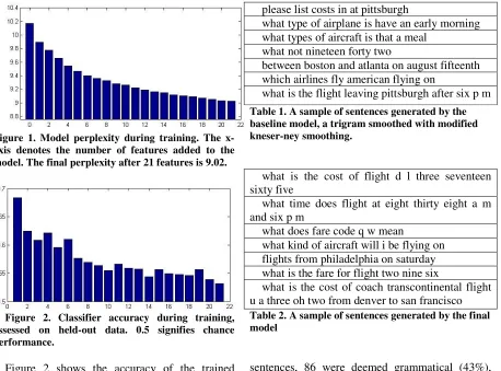
Figure 1. Model perplexity during training. The x-axis denotes the number of features added to the model. The final perplexity after 21 features is 9.02.
Figure 2. Classifier accuracy during training, assessed on held-out data. 0.5 signifies chance performance.
Figure 2 shows the accuracy of the trained features on held-out data. The held-out data was composed of equal parts real and model sentences, so 50% accuracy is chance performance. As might have been expected, the classifiers start out with a relatively high accuracy of 68%, which dwindles down to little over 50% as more features are added to the model. Not surprisingly, there is a strong correlation between the accuracy of a feature and the reduction in perplexity it engenders (spearman correlation coefficient r=0.89, p<10-5.)
In tables 1 and 2 we show a representative sample of sentences from the baseline model and from the final model. As the baseline model is a trigram, it cannot capture dependencies that span a range longer than two words. Hence sentences that start out seemingly in one topic and then veer off to another are common. The global information available to the features used by the boosted model greatly reduces this phenomenon. To get a quantitative sense of this, we generated 200 sentences from each model and submitted them for grammaticality testing by a proficient (though non-native) English speaker. Of the trigram-generated
please list costs in at pittsburgh
what type of airplane is have an early morning what types of aircraft is that a meal
what not nineteen forty two
between boston and atlanta on august fifteenth which airlines fly american flying on
what is the flight leaving pittsburgh after six p m
Table 1. A sample of sentences generated by the baseline model, a trigram smoothed with modified kneser-ney smoothing.
what is the cost of flight d l three seventeen sixty five
what time does flight at eight thirty eight a m and six p m
what does fare code q w mean
what kind of aircraft will i be flying on flights from philadelphia on saturday what is the fare for flight two nine six
[image:6.612.85.543.79.418.2]what is the cost of coach transcontinental flight u a three oh two from denver to san francisco
Table 2. A sample of sentences generated by the final model
sentences, 86 were deemed grammatical (43%), while of those generated by the boosted model 132 were grammatical (66%). This difference is statistically significant with p<10-5.
Finally, let us quantify the computational savings obtained from using rejection sampling. Let |V| stand for the lexicon size (here |V|=603) and |L| for the average sentence length (|L|=14). In Gibbs sampling, a sentence is sampled by starting out with a random sequence of words. For each word position, the current word is replaced with each word in the lexicon, and the probability of the resulting sentence is calculated. Then one of the words is randomly selected for this position in proportion to the calculated probabilities. The sentence has to be scanned in this manner several times for the sample to approximate the model distribution. Assuming we perform only 3 scans for each sentence, Gibbs sampling would have thus required us to classify 3 |V ||L| 25, 000≈
10
7 10⋅ classifications after 21 iterations. In contrast, using rejection sampling, we used only
7
6.7 10⋅ classifications in total – a difference of over three orders of magnitude.
4 Discussion
In this work we presented a method that enables using discriminative learning methods for refining generative language models. Utilizing large- margin classifiers that are trained to discriminate real sentences from model sentences we showed that sizeable improvements in perplexity over a state-of-the-art smoothed trigram are possible.
Our method bears some similarity to the recently developed Contrastive Estimation method (Smith and Eisner, 2004). Contrastive estimation (CE) was proposed as a means for training log-linear prob-abilistic models. As all training methods, contras-tive estimation pushes probability mass unto positive samples. Unlike other methods, CE takes this probability mass from the 'neighborhood' of each positive sample. For example, given a real sentence s, CE might give it more probability by taking away probability from similar sentences which are likely to be ungrammatical, for instance sentences that are formed by taking s and switch-ing the order of two adjacent words in it. This is intuitively similar to our approach – effectively, our model gives probability mass to positive sam-ples, taking it away from sentences classified as model sentences. A major difference between the two approaches, however, is that in CE the defini-tion of the sentence's neighborhood must be speci-fied in advance by the modeler. In our work, the 'neighborhood' is determined automatically and dynamically as learning proceeds, according to the capabilities of the classifiers used.
The sentence representation we chose for this work is rather simple, and was intended primarily to demonstrate the efficacy of our approach. In future work we plan to experiment with richer representations, e.g. including long-range n-grams (Rosenfeld, 1996), class n-grams (Brown et al., 1992), grammatical features (Amaya and Benedy, 2001), etc'.
The main computational bottleneck in our approach is the generation of negative samples from the current model. Rejection sampling allowed us to use computationally intensive
classifiers as our features by reducing the number of classifications that had to be performed during the sampling process. However, if the boosted model strays too far from the baseline P0, these
savings will be negated by the very large sentence rejection probabilities that will ensue. This is likely to be the case when richer representations as suggested above are used, necessitating a return to Gibbs sampling. Therefore, in future work we plan to experiment with classifiers whose decision function is cheaper to compute, such as neural networks and decision trees. Another possible direction would be using the recently proposed Deep Belief Network formalism (Hinton et al., 2006). DBNs utilize semi-linear features which are stacked recursively and thus very efficiently model non-linearities in their data. These have been used in the past for language modeling (Mnih and Hinton, 2007), but not within the whole-sentence framework.
Acknowledgements
We would like to thank Daisuke Okanohara for his generosity in providing the code for the large-margin classifier. The author is supported by the Yeshaya Horowitz association through the center of Complexity Science.
References
Fredy Amaya and Jose Miguel Benedi, 2001, Improve-ment of a whole sentence maximum entropy model us-ing grammatical features. In Proceedings of the 39th Annual Meeting of the Association of Computational Linguistics.
Peter. F. Brown, Vincent. J. Della Pietra, Peter. V. deSouza, Jenifer. C. Lai and Robert. L. Mercer.
Class-based n-gram models of natural language.
Computa-tional Linguistics, 18(4):467–479, Dec. 1992.
Stanley F. Chen and Joshua. Goodman. 1998. An em-pirical study of smoothing techniques for language modeling. Technical Report TR–10–98, Center for Re-search in Computing Technology, Harvard University Stanley F. Chen and Ronald Rosenfeld. 1999a. Efficient sampling and feature selection in whole sentence
maxi-mum entropy language models. In Proceedings of
ICASSP’99. IEEE.
Stanley F. Chen and Ronald Rosenfeld. 1999b. A Gaus-sian prior for smoothing maximum entropy models.
Koby Crammer, Ofer Dekel, Joseph Keshet, Shai Shalev-Shwartz, and Yoram Singer. 2006. Online pas-sive-aggressive algorithms. Journal of Machine Learn-ing Research.
Jianfeng Gao, Hao Yu, Wei Yuan, and Peng Xu. 2005. Minimum sample risk methods for language modeling. In Proc. of HLT/EMNLP.
Charles T. Hemphill, John J. Godfrey and George R. Doddington. 1990. The ATIS Spoken Language
Sys-tems Pilot Corpus. The workshop on speech and natural
language, Morgan Kaufmann.
Geoffrey E. Hinton, Simon Osindero and Yee-Whye Teh, 2006. A fast learning algorithm for deep belief
nets, Neural Computation, 18(7):1527–1554.
Andriy Mnih and Geoffrey E. Hinton. 2007. Three new graphical models for statistical language modeling. In
Proceedings of the 24th international conference on Machine Learning.
Daisuke Okanohara and Jun'ichi Tsujii. 2007. A dis-criminative language model with pseudo-negative
sam-ples. In Proceedings of the 45th Annual Meeting of the
Association of Computational Linguistics.
Brian Roark, Murat Saraclar, and Michael Collins.
2007. Discriminative n-gram language modeling.
Com-puter Speech and Language, 21(2):373–392.
Ronald Rosenfeld. 1996. A maximum entropy approach
to adaptive statistical language modeling. Computer
speech and language, 10:187–228
Ronald Rosenfeld. 1997. A whole sentence maximum
entropy language model. In Proc. of the IEEE Workshop
on Automatic Speech Recognition and Understanding.
Noah A. Smith and Jason Eisner. 2005. Contrastive es-timation: training log-linear models on unlabeled data. In Proceedings of the 43rd Annual Meeting of the Asso-ciation of Computational Linguistics.
Max Welling., Richard Zemel and Geoffrey E. Hinton.
2003. Self-Supervised Boosting. Advances in Neural