Abstract—Biomechanical systems such as horse locomotion are investigated by using inertial sensor systems composed of accelerometers, gyroscopes and magnetometers, or by optical motion tracking systems. The major difficulty in the inertial sensor systems is the integration process. Furthermore, the signals possess noise that has to be filtered. On the other hand, the motion tracking systems are expensive and mostly adapted to indoor laboratory conditions. Hence, in some studies, horses are trained to walk on treadmills with various speeds. This training process is time consuming and may lead to unnatural gaits. In this study, an inexpensive, portable vision system for tracking the motion in a large calibration volume is designed; and an algorithm for obtaining kinematics of a rigid body is developed and implemented in MATLAB. Using the overall system, it is possible to determine the position, velocity and acceleration of any point in the calibration volume which may contain multiple rigid bodies. The point of interest may correspond to points which do not allow an accelerometer to be mounted, or points which are invisible to the cameras. This is the major advantage of our method. A singularity analysis of the algorithm, which yields useful information on the positioning of the markers that are to be tracked by the vision system, is also performed. The method is used to study the whole-body vibrations (WBV) imposed on a horse rider. To the authors’ knowledge, there exists no studies on this topic in the literature. Regarding the imposed WBV, the differences between the gaits of the same horse and the differences between the gaits of different horses (executing the same gait) are investigated. The results are experimentally shown to be consistent with the comfort assessment of four experienced riders.
Index Terms—Horse, inertial sensor system, kinematics, motion tracking, vision system, whole-body vibration
I. INTRODUCTION
HERE are various motivations for investigating the locomotion of horses, such as tracking of trunk movements, detection of lameness, modeling in computer environment and riding simulator constructions [1-5]. In this study, we focus on the vibrations imposed on horse riders. People are exposed to localized or whole-body vibrations during various activities [6]. Horse riders are also exposed to WBV, transmitted through the saddle, which may cause problems such as back pain. Since the response of humans to vibration depends on the vibration frequency, various frequency weighting coefficients are introduced. According
Manuscript received February 06, 2013.
G. Tanil is with the Mechanical Engineering Department, Middle East Technical University, Ankara, TURKEY (e-mail: dgozde@ metu.edu.tr).
R. Soylu is with the Mechanical Engineering Department, Middle East Technical University, Ankara, TURKEY (e-mail: [email protected]).
to BS 6841 and ISO 2631, the coefficients Wband Wk are used for the vertical direction, respectively. Wd, on the other hand, is used for the lateral and fore-aft directions [7-8].
To assess the effects of vibrations on the human body, the acceleration of the point(s) at which the person is in contact with the source needs to be determined. Inertial sensor systems are the conventional means of measuring these accelerations. Also, WBV Dosimeter and Analyzer can be used to compute various WBV indicators which are generally based on the acceleration of a single point, whose location does affect the values of the measurements. The effect of different seat-back angles and different accelerometer heights on the vibrations imposed on the driver of a sports vehicle is investigated in [9].The authors performed the experiments various times along the same road by positioning the accelerometer at different heights at each trip. Clearly, the experiment could be completed in a single trip by using multiple accelerometers. However, due to the size of the seat pad containing the accelerometer, it was possible to make only one measurement in a trip. Even if one uses expensive, custom-made accelerometers to avoid this restriction, the weight and size of the accelerometers still may impose constraints on the positioning of them [10]. Furthermore, in some cases, accelerometers cannot be used to measure the accelerations of the desired points because the points of interest are not suitable for mounting an accelerometer, or the points are too close to each other. On the other hand, if the velocity and position of the points are of interest, the acceleration data obtained via accelerometers should be integrated. This may lead to inaccurate results due to accumulation of integration errors.
Alternatively, a vision system may be used such that the position vectors of the points of interest are tracked by mounting markers [11-13].After filtering the position data appropriately, one may obtain the velocity and acceleration vectors of the markers by differentiation. Similar to the case where accelerometers are used, filtering or smoothing techniques are again necessary, since differentiation tends to amplify the measurement noise [14].
In this study, we developed a portable vision system composed of 3 off-the-shelf cameras with a speed of 30 fps and a resolution of 640 x 480 pixels at video mode. The system costs about $300 and can be efficiently used for motion tracking purposes. Indeed, there are sophisticated motion capture systems, such as VICON, SIMI, etc, which employ 6-8 high resolution and high speed cameras. These systems are also equipped with special software. However, they are not easily portable and they cost $20.000- $75.000.
A Vision Based Approach for Assessing Equine
Locomotion and Whole-Body Vibration Induced
on a Horse Rider
Gözde Tan
ı
l (Do
ğ
an) and Re
ş
it Soylu
Fig. 1. (a) The calibration board on the mechanism and its degree of freedom. (b) The vision system located in manege. The calibration volume is shown in the rectangular prism. Dimensions are in mm.
When a motion or scene is recorded by two cameras, one obtains 3D (3 dimensional) data which involves depth information as well [15]. Our system consists of 3 cameras to obtain more accurate results compared to a stereo system. The relationship between the 2D image coordinates and the 3D world coordinates depends on the intrinsic and extrinsic parameters of the cameras which are obtained via camera calibration. Only radial distortions are modeled and a planar pattern is proposed within the calibration volume as a model to be observed by the cameras [16]. A calibration technique compensating for both the radial and tangential distortions is also suggested [17]. As motivated from these studies, a MATLABcamera calibration toolbox is developed [18]. In our study, a planar, checkerboard patterned calibration board and a positioning mechanism are designed and manufactured. This mechanism has two rotational degrees of freedom and is mounted on a four-wheel chassis to provide the translational freedom necessary for the unusually large calibration volume as required in our study as shown in Fig. 1(a).
Here, we show that a vision system may be efficiently used to measure the acceleration of points on a rigid body by tracking only 3 markers on the body. This is practically equivalent to mounting various accelerometers on that body. The accelerations of points which are invisible to the cameras, or, accelerations of points on different bodies may also be obtained. Vibration indicators may then be computed using the acceleration of any point on any body.
For the experimental demonstration, the WBV induced on a horse rider is considered. Vibrations, imposed by different horses and different gaits, are quantified using the developed vision system. This quantification leads to various, novel horse comfort indicators. Using 4 horses, the indicators are experimentally shown to be consistent with the comfort assessment of 4 experienced riders. The differences between the gaits of the same horse and the gaits of different horses executing the same gait are also investigated.
In order to determine the vibrations induced on the rider, 3 passive markers, made of special 3M® tape, are attached to
the body of the horse such that the markers are as close as possible to the saddle. The saddle and markers, which is the source of vibrations for the rider, constitute the so-called Rigid Body of Interest, RBI. The motion of the horses is then recorded with the developed system. The movies are extracted into image frames by the AVD Video Processor. In order to obtain the coordinates of the tracked markers, the images are processed by various algorithms based on image processing techniques [19]. Thus, the position vector of each marker is obtained in one camera reference frame. After smoothing the position data of each marker, in order to take
full advantage of the periodicity of the motion, the position vector is transformed into a more convenient reference frame named as the motion reference frame (MRF). Next, the rigid body constraints are enforced on the markers since they are on the same rigid body. For this purpose, the 3D object registration algorithm is used [20]. Fourier functions of optimal orders are then used to approximate the 2 periodic components of each marker position vector. These functions are analytically differentiated to obtain the velocity and acceleration vectors for each marker. Knowing the velocity and acceleration vectors, the angular velocity and acceleration vectors of the RBI are computed. Finally, the acceleration of any point on the RBI is calculated, the singularities of which are also analyzed.
II. MATERIALS AND METHODS
A. The Vision System and Calibration
The developed vision system is composed of 3 Casio®
Ex-Z750 cameras that are synchronized by a flashlight. The highest resolution at the video mode is 640 × 480 pixels and the frame rate is 30 fps. Actually, these are typical values for most off-the-shelf cameras. Slightly more expensive high speed cameras have also been considered for our system. However, it has been observed that as the frame rate increases, the resolution decreases and becomes inadequate for our experiments. The cameras are 7.5 meters far from the experiment scene and they can record a volume of 6.45 m × 0.7 m × 0.5 m as shown in Fig. 1(b).
In order to obtain the 3D position of any point within the calibration volume, the intrinsic and extrinsic parameters of the cameras are required. Determination of these parameters is known as camera calibration. The intrinsic parameters are the physical characteristics of a camera that relate the camera reference frame (CRF) to the image reference frame. The extrinsic camera parameters RBA (rotation matrix
between A and B) and tBA (translation vector between A and
B) relate the two camera reference frames A and B via
r(A) R
B Ar(B) t
B
A (1)
where r(A)and r(B)are the position vectors of a point
expressed in the CRF of camera A, i.e., CRF(A), and CRF of camera B, i.e., CRF(B). The calibration toolbox is used both for the calibration of each camera and each pair of cameras [18]. The three cameras lead to three camera pairs as left & middle, left & right and middle & right. Hence, the extrinsic parameters consist of three rotation matrices and three translation vectors. For the calibration process, a calibration board of size 800 mm × 1500 mm, covered by a checkerboard pattern of 50 mm × 50 mm squares, is prepared. Fig. 1(a) shows the mechanism to orient and translate the calibration board. The calibration images consist of 90 images of the calibration board at 90 different homogeneously distributed positions and orientations.
B. Marker Identification via Image Processing
[image:2.595.49.291.51.147.2]image, each element of the image is a 3D vector. The components of this vector correspond to red, green and blue for the RGB model. Images can be transformed from one type to another by transformation. In this study, the coordinates of the tracked markers are obtained by processing the images via various algorithms.
After various trials based on the visibility of the markers, the diameter of the markers attached to the horses is chosen to be 60 mm. A light source of 1000W is directed to the markers so that the silver-gray color of the markers appears as white as possible. After converting the color images to grayscale, they are converted to binary by a user specified threshold value. The purpose here is to keep the regions that are white. However, besides the markers, there may be other white regions. Therefore, additional filtering methods are required to identify the markers. First, in the whole image plane, an area filter is introduced to eliminate the white regions which are either too small, or too large compared to a marker, the area of which is computed using the first frame of the related video. The remaining filters, namely the
distance and cross product filters, are computationally
expensive to apply. Hence, to reduce the execution time, a dynamic window is introduced such that these filters are applied to the white regions inside this window only. For this purpose, the 3 markers are identified in the first image and the centroid of these, Wce 1 is determined. Here, Wce k denotes the overall geometric center of the 3 markers
in frame k. Using the first image, an appropriate width, Wdu,
and height,Wdv, are selected for the window (see Fig. 2). In
the second frame, the distance and cross product filters are applied only to the regions inside the window whose center, width and height are Wc (2), Wdu and Wdv respectively,
where Wc k Wce k–1 . The process is applied
automatically to the remaining frames of the motion, making the window slide as the overall marker center moves.
The distance filter is introduced to get rid of noisy regions in the window as shown in Fig. 3(a). Let the number of white regions in the window be Nw and the number of markers be Nm. Furthermore, let
drs= ur–us 2
+ vr–vs 2 1/2
(2) denote the distance between the centroids of the regions labeled as r and s, where (ur, vr) and (us,vs) are the image coordinates of these regions. Consider, Nm =3 white regions,
i, j and k, in the window and let the distances between centroids of these regions be dij, dikand djk. These regions will pass the distance filter (i.e., i, j and kmay correspond to markers 1, 2 and 3, respectively) if and only if the condition
|r12|(1–ε12)≤dij ≤|r12|(1+ε12)] |r13|(1–ε13)≤dik
≤|r13|(1+ε13)] |r23|(1–ε23)≤djk ≤|r23|(1+ε23)] (3)
is satisfied where, rpq is the distance between the centroids
[image:3.595.305.553.50.218.2]of markers p and q obtained from the first frame of the motion. Here, εpq is a user specified, allowable percent error for dpq. Note that there are C(Nw, Nm)=Nw! / [Nm!(Nw–Nm)!] combinations of picking Nm out of the Nw regions in the window. Each of the C(Nw,Nm) possibilities, and their permutations, should be processed by this filter.
Fig. 2. Window operation between frames k and k–1.
Fig. 3. (a) A sample of regions that needs distance filtering (b) An example for the cross product filtering
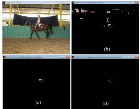
Fig. 4. The stages of filtering methods applied to Horse 3 - walk. The centers of the regions are shown by red asterisk (a) The original RGB color image (b) The area filtered black and white image (c) The regions in the dynamic window (d) The distance and cross product filtered image
Next, for the noises still occurring due to the pseudo markers passing the distance filter, the cross product filter is introduced. In Fig. 3(b), there exist two choices for the second marker (regions 2 and 2') both of which pass the distance filter. The correct position of the second marker is region 2 if and only if sgn [(r12×r23)3] in the considered
frame equals to sgn [(r12×r23)3] in the first frame (known).
Here, sgn is the sign operator, rij is the vector from marker i
to j and (..)3 is the 3rd component of the vector in the
parenthesis. A sample of the sequential applications of the proposed filters is shown in Fig. 4.
C. From Image to 3D Data (Smoothing, Reference Frame
Transformations, Registration and Curve Fitting)
After obtaining the image coordinates of the marker centroids, the 3D positions of the markers are obtained by the transformation function provided in [18]. The position vector of each marker, in the 3 different camera pairs, is then expressed in the left camera reference frame, CRF(L). These 3 vectors, which need to be identical, are not identical in practice due to calibration errors, resolution of the cameras, etc. However, the three vectors are quite close to each other and the average of them is taken to be the true position vector of the marker.
[image:3.595.312.539.240.417.2](b) filtering functions of MATLAB, each component of each
marker’s position vector is smoothed. Next, in order to take the full advantage of the periodicity of the saddle motion, the position vectors are expressed in a more convenient reference frame, called the Motion Reference Frame. The x,
y and z axes of the MRF are expressed by the unit vectors u1M, u2M and u3M, respectively. u1M is in the
direction of the net displacement (taken in two periods of motion) of one of the markers chosen by the user. Denoting the position vector of the selected marker by r and the period of motion byT, u1M is obtained as
u1M
=
r|t 2T–r|t 0r|t 2T–r|t 0 (4)
The second unit vector of the MRF corresponds to the gravity direction, which is obtained by a plumb marked by 2 markers. At this step, a correction algorithm is employed since the angle between u1M and the estimated gravity
vector, u2eM, cannot be obtained exactly as 90°, although very close to this value. The third unit vector of the MRF is obtained via
u3M = u1M u2M
e
u1M u2eM (5)
Finally, having obtained u1M and u3M, the corrected
gravity vector, u2M, is obtained by the cross product u3M u1M. Therefore, the relation between CRF(L) and
MRF is given by the rotation matrix
RM L u1M (L) |u2M (L) | u3M (L) (6)
such that
r(M) R
M
L -1 (L) (7)
where r(M) and (L)denote the position vector r expressed in
the MRF and CRF(L), respectively.
The developed methods are illustrated using Horse 2 while it is cantering. In Fig. 5(a), the components of the position vectors of the 3 markers, in CRF (L), are given for two periods of motion. Fig. 5(b) shows the smoothed components in the MRF where the periodic nature of the motion is more apparent.
In this study, it is assumed that the saddle is firmly attached to the horse and the skin movements are negligible compared to the overall motion of the horse. Therefore, the so-called Rigid Body of Interest (RBI) is composed of the contact point on the saddle, which is invisible to cameras, and the 3 markers attached to the horse. A 3D registration/ correction algorithm is employed to ensure that the rigid body constraints are satisfied by the 3 markers which are located as close to the contact point as the constraints allow [20]. Application of this algorithm ensures the best alignment of a measured data set with a model data set. Here, the model data (rj m) denotes the position vector of
marker j obtained in a frame of static pose and measured data (rj) is the position vector of marker j obtained during
the motion. The registration algorithm used is based on the minimization of the error function
e(q)=1
M rj
m R q
R rj qt 2 M
j=1 (8)
where M (=Nm=3, here) is the number of the data (markers) to be registered. R is a rotation matrix relating the model and the measured data sets; q [qR|qt where qt
[q4q5q6 is a unit quaternion representing the translation between the model and measured data sets and qR
[q0q1q2q3 is a unit quaternion representing the rotation matrix R via
2 2 2 2
0 1 2 3 1 2 0 3 1 3 0 2
2 2 2 2
1 2 0 3 0 2 1 3 2 3 0 1
2 2 2 2
1 3 0 2 2 3 0 1 0 3 1 2
2( ) 2( )
2( ) 2( )
2( ) 2( )
q q q q q q q q q q q q
q q q q q q q q q q q q
q q q q q q q q q q q q
⎡ + − − − + ⎤
⎢ ⎥
=⎢ + + − − − ⎥
⎢ − + + − − ⎥
⎣ ⎦
R
(9)
Minimizing e(q) with respect to q gives the registered position vector of marker j as
rjr Ropt qR
–1
(rj m qtopt (10)
where Ropt and qtopt are the optimal values of R and q t at
each frame of the motion. The next task is to determine the velocity vector, vj, and acceleration vector, aj, of marker j
where j = 1, 2, 3. This is achieved by finding an optimal function minimizing the error ∑t=tmax
t=0 [gj t-gj
fit t ]2 to approximate each component of rjr. Here, gj t denotes x, y or z component of rjr and gj
[image:4.595.315.538.405.770.2]fit t is the function fitted to g j t with undetermined coefficients. Finally t denotes discretized time given by t k–1/fps where k and fps denote frame number and frames per second, respectively.
Fig. 5. Positions of the 3 markers in (a) CRF(L) (b) MRF (Horse 2-canter)
0 10 20 30 40
-5000 0 5000
Horse 2 Canter
3 markers in Left Camera Reference Frame
X c
oo
rdi
nat
e
s
[m
m
]
marker 1
marker 2 marker 3
0 10 20 30 40
-400 -200 0 200
Y c
oo
rdi
na
te
s
[
m
m
]
0 10 20 30 40
8000 8500 9000
number of frames
Z
c
oor
di
na
tes
[m
m
]
0 0.2 0.4 0.6 0.8 1 1.2
-5 0 5
x c
oord
ina
te
s
[m
]
Horse 2 Canter 3 markers in Motion Reference Frame marker 1
marker 2 marker 3
0 0.2 0.4 0.6 0.8 1 1.2
-0.6 -0.4 -0.2 0
y
co
ord
inat
es
[m
]
0 0.2 0.4 0.6 0.8 1 1.2
-8.6 -8.4 -8.2
seconds
z
coo
rdi
nat
es
[m
]
Fig. 6. The options for the curve fitted position of 1st marker in y axis (Horse 2-canter) and its derivatives
In order not to violate the rigid body constraints assured by the registration algorithm, curve fitting is applied to the position data in order only to obtain velocity and acceleration of marker j. That is, the position of marker j
will finally be represented by rjr, not gj
fit t. Each component of vj and aj, on the other hand, are represented by gjfit t and gjfit t , respectively. The velocity of the horse in the x
direction is considered to be constant, indicating that a linear polynomial for the x component of rjr can be selected. On
the other hand, for the y and z components, gjfit t is selected to be a Fourier series given by
gfitj t a0+∑Nn=1ancos (nωt) +bnsin (nωt) (11)
where, ω: fundamental frequency; N: number of harmonics;
a0, an and bn: undetermined coefficients. Here, N is a
selectable parameter, the optimum value of which, Nopt, can
be obtained by the method proposed in Appendix A. Firstly, the number of extremes, E, is determined by counting the maxima and minima of the displayed gj(t) plot. The fact proved in Appendix A indicates that the minimum order of the Fourier series to be fitted must be E/2 to account for all of the extremes. Hence, two alternative Fourier fits, with degrees (E/2) and [(E/2) + 1], are graphically presented to the user in order to determine Nopt by observing the graphs
and the numerical goodness of the fits. For example, Fig. 6 shows the 2 Fourier functions, of orders 2 and 3, proposed by the program to approximate the y component of the first marker with E=4.
D. The Angular Velocity and Acceleration of the RBI
Once the position, velocity and acceleration vectors of 3 points on a rigid body are known, the angular velocity (ω) and acceleration (α) of the RBI may be computed. To compute ω,firstly, v1 is expressed in terms of v2 and v3 by the following consistent equations
v1 v2 ω r21 (12)
v1 v3 ω r31 (13)
where rij rj – ri is the relative position vector of marker j with respect to i andvj is the velocity of marker j. Equations (12) and (13) may be solved for ω using Appendix B by taking K1 , K2 , K3 and K4 to be r21, (v2–v1), r31 and (v3–v1),
respectively. Using (B6) and (B7), the 2 solutions for ω are given by
ω1 v2 v1 v3 v1
r31·v2 v1 (14)
ω2 v2 v1 v3 v1
r21·v3 v1 (15)
provided that the denominators are nonzero. Also, the compatibility condition given by (B8) yields
r21· v3 v1 v2 v1 · r31 (16)
which may be written as
r21· v3 r21· v1 r31· v2 r31· v1 0 (17)
Since markers 1 & 2, and 1 & 3 are on the same RBI, the following two conditions should be satisfied.
r21· v1 r21· v2 (18)
r31· v1 r31· v3 (19) Substituting (18) and (19) into (17) and simplifying
r21 r31 · v3 v2 0 (20)
Since r21 r31 r23, (20) becomes
r23· v3 v2 0 (21)
which is always true, since markers 2 & 3 are on the same RBI. Hence, we show that the compatibility condition given by (16) is always satisfied and (12) and (13) lead to a unique solution for ω.
Singularity check: To investigate the case where the
denominator of (14) is zero, ω1 is written as ω1 ω r21 ω r31
r31· ω r21 (22)
which is obtained by solving v2 v1 and v3 v1 from (12)
and (13) and substituting into (14). After simplification, ω1 ω · r21 r31 ω
r21 r31· ω (23)
Let us define the unit normal vector, n,of the plane formed by the 3 markers, via the equation
n (r21 r31)/ c (24)
where c |r21 r31|. Note that c 0 provided that the 3
markers are not collinear. Solving (r21 r31 from (24) and
substituting the result in (23), we obtain
ω1 ωn ·cn· ωc ω
(25) The denominator of ω1 will be zero iff ω·n 0, which also makes the numerator zero as well. Hence, if the angle between ω and n is 90°, or 270°, the solution for ω1 will be
singular. Hence, in order to avoid this singularity, n and ω should be prevented from being perpendicular to each other. Ideally, ω1 and ω2 should be identical. However, the
errors associated with the vision system, the curve fitting operations, etc, cause them to vary in practice. Also, v1 has been expressed in terms of v2 & v3 in the above formulation. Alternatively, one can express v2 in terms of v1 & v3,or, express v3 in terms of v1 & v2. Hence, totally 6 values are obtained for ω. In our program, time plots of all 6 angular velocities are displayed, any of which may be discarded by
0 0.5 1
-0.4 -0.3 -0.2 -0.1
Horse2 Canter-marker 1 Fourier2
P
o
si
tio
n
in
y
[m]
seconds
T = 0.6 s
0 0.5 1
-10 0 10
5
-5
seconds
V
el
oc
ity
[
m
/s
]
A
cc
ele
ra
tio
n
[m
/s
2]
0 0.5 1
-0.4 -0.3 -0.2 -0.1
seconds
Horse2 Canter-marker 1 Fourier3
T = 0.6 s registered curve fitted
0 0.5 1
-10 0 10
5
-5
seconds
the user. The average of the accepted values is used in further calculations.
The angular acceleration of the RBI is obtained by firstly expressing a1 in terms of a2 & a3 via the equations
a1 a2 ω ω r21 α r21 (26) a1 a3 ω ω r31 α r31 (27)
where aj is the acceleration vector of marker j and α is the angular acceleration of the RBI, which is to be found. It is assumed that the angular velocity ω is obtained using the above approach. The two solutions for ,obtained by using Appendix B, are given by
1 a2+ω ω r21 a1 a3+ω ω r31 a1
a2+ω ω r21 a1 · r31 and
2 a2+ω ω r21 a1 a3+ω ω r31 a1
r21 ·a3+ω ω r31 a1 (28)
The singularity associated with the angular acceleration is the same as for the angular velocity.i.e., n and αshould not be perpendicular.
E. Acceleration of Any Point on the RBI
Since the position, velocity and acceleration of 3 points on the RBI; and the angular velocity and acceleration of the RBI are known, the position, velocity and acceleration of any point on the RBI can be computed. Consider, for instance, the saddle marker, S, which is invisible to the cameras during riding. Using the frame of static pose of the horse without the rider, the saddle marker position can always be obtained in the body reference frame (BRF) shown in Fig. 7.
Here, the origin, OB, of the BRF is selected to be at the center of marker 1 and marker 2 lies on the positive xB axis. The unit vectors u1B, u2B, and u3B are parallel to the xB, yB, zB axes of the BRF. These vectors can be determined via
u1B(M) r2(M) r1(M)
|r2(M) r
1
(M) | ; u2B(M)
r3(M) r1(M)
|r3(M) r
1 (M) |
u3B(M) u1(MB) u2(MB)
|u1(MB) u2(MB)| ; u2B
(M) = u 3B
(M) u
1B (M) (29)
where a superscript M indicates that the vector is expressed in the MRF. Therefore, the rotation matrix, RB Mrelating BRF
and MRF is obtained as
RB M u1B(M)|u2B(M)|u3B(M) (30)
From Fig. 7 it follows that
rS(M) r1(M) r1S(M) (31) where rS(M) is determined using the static shot. Substituting
r1S(M) RB Mr1S(B) into (31) and solving for r1S(B)
r1S(B) RB M r
S
(M) r
1
(M) (32)
Finally, the position vector of S, rS, may be obtained via
rS(M) RB Mr 1S
(B) r
1
(M) (33)
Here, RB M and r1(M) depend on time, but r1S(B) is constant.
The velocity and accelerationof the saddle marker S, vS and
aS may be obtained in terms of the velocity and acceleration of any of the 3 markers.
' B
y
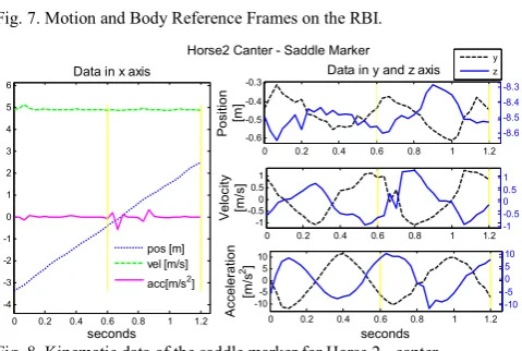
Fig. 7. Motion and Body Reference Frames on the RBI.
Fig. 8. Kinematic data of the saddle marker for Horse 2 - canter
In the case of no measurement errors, the 3 alternative expressions obtained for vS (or aS) should be identical. Since slight differences may occur, one can take vS (or aS) to be the average of the 3 results, e.g. using marker 1, the velocity and accelerationof the marker S, expressed in the MRF are
vS(M) v1(M) ω(M) r
1S
(M) (34)
aS(M) a1(M) ω(M) ω(M) r
1S
(M) (M) r
[image:6.595.307.547.144.305.2]1S (M) (35)
Fig. 8 shows the position, velocity and acceleration components of the invisible saddle marker S on Horse 2 while cantering.
F. Whole-Body Vibration
The x component of the acceleration of the saddle marker in the MRF is approximately zero due to the constant average velocity, Vx,avg, while the y and z components are
obtained to be periodic. Since the accelerations along the y
and z axis are observed to be significant for the motion of the rider, the overall acceleration has been considered while assessing the effects of WBV. Therefore, the weighted accelerations in the vertical and lateral directions are computed to obtain the overall acceleration. For our computations, the weighting coefficients Wb, Wd and Wk are required. The weighting coefficients provided are in the form of transfer functions [21]. Hence, the closed form expressions for Wb, Wd and Wk, which do not exist in the available literature to the authors’ knowledge, are generated by MATHEMATICA. The results are given as
9 2 2 -6 4
-8 6 13 12 2
15 4 13 6 12 8
= 1.8018 10 sqrt((0.0001 - 0.00001 + 2.6196 10
+ 1.0428 10 )/(4.2949 10 - 2.1752 10 + 1.6778 10 - 8.4971 10 + 6.1021 10 + 3.20
b
W f f f
f f
f f f
⋅ ⋅ ⋅ ⋅ ⋅ ⋅
⋅ ⋅ ⋅ ⋅ ⋅
⋅ ⋅ ⋅ ⋅ ⋅ ⋅
10 10 8 12 14 16
0 10⋅ ⋅f + 1.0006 10⋅ ⋅f + 320.0095⋅f + f ))
(36)
9 2 -6 2 -6 4
-8 6 12 11 2 14 4
13 6 12 8 9 10 8
=1.2240 10 ×sqrt((0.00005 - 6.9232 10 + 1.5829 10 + 1.0428 10 )/(7.4120 10 - 5.1469 10 +2.8959 10 - 2.0105 10 + 2.3832 10 +7.2544 10 + 1.0002 10
k
W f f f
f f f
f f f
⋅ ⋅ ⋅ ⋅ ⋅ ⋅
⋅ ⋅ ⋅ ⋅ ⋅ ⋅ ⋅
⋅ ⋅ ⋅ ⋅ ⋅ ⋅ ⋅ 12
14 16
+72.5465 + ))
f
f f
⋅
⋅ (37)
8 2 4
11 4 2
4 2
= (1.9585 10 )/sqrt(((39.8987 + 1558.5454 ) ( 1.5585 10 + 1558.5454 ) (24936.7273 + 3238.8215 + 1558.5454 ))/( 157.9136 + 39.4784 ))
d
W f f
f f
f f
⋅ ⋅ ⋅
⋅ ⋅ ⋅ ⋅ ⋅
⋅ ⋅ (38)
0 0.2 0.4 0.6 0.8 1 1.2
-4 -3 -2 -1 0 1 2 3 4 5 6
Data in x axis
seconds
pos [m] vel [m/s] acc[m/s2]
0 0.2 0.4 0.6 0.8 1 1.2
-0.6 -0.5 -0.4
-0.3 Data in y and z axis
Po
si
tio
n
[m]
-8.6 -8.5 -8.4 -8.3
y z
0 0.2 0.4 0.6 0.8 1 1.2
-1 -0.5 0 0.5 1
Ve
lo
ci
ty
[m/s]
-1 -0.5 0 0.5 1
0 0.2 0.4 0.6 0.8 1 1.2
-10 -5 0 5 10
A
cceler
ation
[m/s
2]
seconds
where, f denotes frequency. Next, commonly used WBV indicators (See Table I) are computed. The total, daily allowable values regarding atotal,W,rms is denoted by A(8). EU
Physical Agents Directive defines Exposure Action Value (EAV) as the limit of the acceleration value that a person can be exposed to vibration without health damage; and Exposure Limit Value (ELV) as the acceleration value above which the person is exposed to health risks. The numerical values for A(8) is 0.5 m/s2 (EAV) and 1.15 m/s2 (ELV). VDV values are not considered, since the crest factors in each axis are obtained as less than 6. We define the allowable duration [hr] to reach the A(8) threshold by
TA(8),W and allowable daily distance [km] that can be covered
by DA(8),W. Definitions of these novel vibration indicators are
given below.
TA 8 ,W 8 a A(8)
total, W,rms and DA 8 ,W =Vx,avgTA 8 ,W (39)
TA(8),W and DA(8),W may be used as a measure of the
comfort level of a horse and/or gait. These indicators are presented in Table II for Horse 2 (canter) by considering the BS 6841 and ISO 2631 definitions.
III. RESULTS OF THE EXPERIMENTAL STUDIES & DISCUSSION
The whole procedure has been applied to the 4 horses in 3 gaits i.e. walk, trot (sitting-rising) and canter. The features of the horses are given in Table III.
The average velocities of the horses are obtained as 4.5-5 km/h (walk), 8.7-10.5 km/h (trot) and 16.7-18.3 km/h (canter). Fig. 9 shows the results for a horse at walk and another horse in sitting trot. The results for the all gait and horse combinations can be found in [22].
TABLE I
DEFINITIONS OF VIBRATION INDICATORS
Symbol Vibration indicator Formula
AW(t) Weighted acceleration W·A(t)
aW,rms
Weighted root mean square acceleration
1
τ AW 2(t)
τ
0 dt
aW,peak Weighted peak acceleration max[abs(AW(t))]
CF factorCrest ,
,
W peak
W rms a
a
atotal,BS,rms
Overall weighted RMS acceleration (BS 6841)
ax,Wd,2 rms+a
y,Wb,rms
2 +a
z,Wd,rms 2
atotal,ISO,rms
Overall weighted RMS acceleration
(ISO 2631) (1.4ax,Wd,rms) 2+a
y,Wb,rms 2 +(1.4a
z,Wd,rms)2
VDVW
Weighted vibration dose
value AW 4(t)dt
τ
0
4
TABLE II
VIBRATION INDICATORS FOR HORSE2(CANTER)
Indicator BS6841 ISO 2631 Unit
ay,Wb,rms 3.191 - m/s2
ay,Wk,rms - 3.701 m/s2
az,Wd,rms 6.119 6.119 m/s2
atotal,W,rms 6.901 9.331 m/s2
TA(8),W, action 0.042 0.022 hr
TA(8),W, limit 0.222 0.121 hr
DA(8),W,action 0.741 0.405 km
DA(8),W,limit 3.919 2.143 km
In Fig. 10, the overall weighted RMS acceleration versus gait style plots are given for the 4 horses considering BS 6841. Clearly, the acceleration increases as the walking style changes from walk to sitting trot and canter. The trend of the change is shown by the dashed lines, which disregard the rising trot since the rider’s seat is in contact with the saddle only momentarily in this style of riding. For the 4 horses, the allowable time versus gait style and the allowable distance versus gait style plots are given in Fig. 11 and Fig. 12, respectively. As expected, the time limitations are larger in walk, compared to the remaining gaits. Although the time limitations for sitting trot and canter are close to each other, the limitation for sitting trot is higher for each horse. Similarly, the allowable distance in the walk is high.
TABLE III
HORSES TAKING PART IN THE EXPERIMENTS
Feature H 1 H 2 H 3 H 4
Breed German Dutch French English
Age 20 10 19 13
[image:7.595.305.539.593.782.2]Height at withers [m] 1.70 1.73 1.58 1.57
Fig. 9. Kinematic data of the saddle marker (Horse 1-walk) & (Horse4-trot)
Fig. 10. atotal,W,rmsvs gait style for 4 horses.
Fig. 11. TA(8),W, limit vs gait style for 4 horses, i.e. allowable riding time.
0 0.5 1 1.5 2 2.5
-2 -1.5 -1 -0.5 0 0.5 1 1.5 2
Data in x axis
seconds pos [m] vel [m/s] acc[m/s2]
0 0.5 1 1.5 2 2.5
-0.6 -0.55 -0.5 -0.45
Data in y and z axis
Pos iti on [m ] -6.65 -6.55 -6.45 y z
0 0.5 1 1.5 2 2.5
-0.4 -0.2 0 0.2 0.4 Vel oc ity [m /s ] -0.6 -0.3 0 0.3 0.6
0 0.5 1 1.5 2 2.5
-6 -3.5 -1 1.54 A ccel er at ion [m /s 2] seconds -10 -7.5 -5 -2.5 0 2.5 5 7.5 Horse1 Walk - Saddle Marker
0 0.5 1
-2.5 -2 -1.5 -1 -0.5 0 0.5 1 1.5 2 2.5
Data in x axis
seconds pos(m) vel(m/s) acc(m/s2)
0 0.2 0.4 0.6 0.8 1 1.2 1.4
-0.36 -0.34 -0.32 -0.3 -0.28
Data in y and z axis
Po si tio n [m ] -6.7 -6.65 -6.6 -6.55 -6.5 y z
0 0.2 0.4 0.6 0.8 1 1.2 1.4
-0.4 0 0.4 0.8 Vel oc ity [m /s ] -1 -0.5 0 0.5 1
0 0.2 0.4 0.6 0.8 1 1.2 1.4
-18 -12 -6 0 6 Acc el er at io n [m /s 2] seconds -12 -6 0 6 12 18 24 Horse4 Sitting trot - Saddle Marker
0 5 10 15 Horse 1 O ve rall W e ig ht ed R M S A cc . [m /s 2 ]
walk sitting trot rising trot canter
0 5 10 15 Horse 2 0 5 10 15 Horse 3 0 5 10 15 Horse 4 0 0.5
1 Horse 1
Al lo w a bl e R idi ng T im e [ hr ]
walk sitting trot rising trot canter
0 0.5
1 Horse 2
0 0.5
1 Horse 3
0 0.5
1 Horse 4
(a)
Fig. 12. DA(8),W,limit vs gait style for 4 horses, i.e. allowable riding distance.
Fig. 13. The relationship between the vibration indicators and comfort grades for sitting trot (1:very bad, 2: bad, 3: medium, 4: good, 5: very good)
However, for the sitting trot and canter, the difference changes for each horse, since velocity of the horse affects the distance. During the experiments, each rider graded each horse, in all gaits to assess the comfort level. In Fig. 13, relations between the vibration indicators and comfort grades are shown for sitting trot. The results for all indicators considering only vertical vibrations, neglecting the lateral, are given in [23]. The average of the riders’ comfort grades for the all horse gaits are given in Table IV.
Accuracy of the vision setup for position and acceleration
Since the position of markers is the first data obtained by our setup, the accuracy of the position data is tested. For this purpose, various points on the calibration board are considered. The distances between these points are measured by an accurate caliper and by the system. The errors associated with the measured distance data on the calibration board vary between 2 and 5 %.
Since the basic concern in our study is acceleration, the setup is used to determine the gravitational acceleration. A tennis ball of diameter 65 mm, covered by retroreflective 3M®, is tracked during a free fall. The coordinates of the ball center are obtained via image processing. The position vector is obtained for 21 image frames (lasting 0.7 s). Since the acceleration in the gravity direction is sought for, a unit vector showing the gravity direction is obtained via a plumb. The position of the ball in the gravity direction is obtained by the dot product of the position vector of the ball with the unit vector along the gravity direction. A quadratic polynomial is fitted to the position, since the acceleration is expected to be constant. Next, the gravitational acceleration is obtained by differentiating the position twice. The gravitational acceleration is calculated to be 9.5 m/s2, i.e.
with an error of 3.6 %, when air resistance is neglected. TABLE IV
AVERAGE OF THE RIDERS’COMFORT GRADES FOR THE HORSE GAITS
(1: very bad, 2: bad, 3: medium, 4: good, 5: very good)
Gait Style H 1 H 2 H 3 H 4
Walk 3.75 4.50 4.25 2.75
Sitting trot 2.50 4.00 4.00 2.00 Rising trot 3.00 4.50 4.25 3.00
Canter 2.75 4.75 5.00 2.25
Average of 4 gaits 3.00 4.44 4.38 2.50
One of the objectives of this study is to demonstrate that inexpensive cameras may be used to construct a vision system which can be used in outdoor applications, rather than the limited space of laboratories. Although the cameras used in this system are inexpensive, their frame rates and resolutions are low. Hence, the quality of the cameras is the main source of error in our results. This error may be easily eliminated by using superior cameras. Such a replacement can be realized at affordable costs. For instance, it is possible to buy a 30-1000 fps camera with a resolution of 1280 × 720 to 224 × 64 (at video mode) at a price of 300$.
The allowable distance and time values obtained in this article are based on the ELV as specified by the EU Physical Agents Directive. These values are over-safe because, the ELV values used assume that the person subjected to vibrations is totally passive. In the case of riding, however, the rider compensates for the induced vibrations. For instance, in sitting trot, the rider moves his belly like a belly dancer. In the case of canter, the rider moves as if he is swinging. Therefore, the vibration indicators determined in this study should be interpreted as relative, rather than
absolute indicators.
IV. CONCLUSION
In this study, a modular vision system, which consists of 3 inexpensive cameras, has been developed to track passive markers. Efficient filters are developed in order to identify the markers in the images. The components of the position vector of the markers are optimally smoothed in order to ensure that noise is not amplified during differentiation. For the markers that belong to the same rigid body, rigid body constraints are taken into account via the registration algorithm. Hence, the errors in the position data due to the violation of these constraints have been, at least partially, compensated. Such violations may occur, for instance, due to the movement of the skin on which a marker is mounted.
The velocity and acceleration vectors of markers are obtained by differentiating the position vector. The outputs of the vision system are the position, velocity and acceleration vectors of the tracked markers. These outputs are the inputs of the developed algorithm which computes the position, velocity and acceleration vectors of any point on a rigid body which possesses at least 3 tracked markers. The performed singularity analysis of the algorithm reveals the optimal location of the markers. The markers should be positioned such that the angular velocity and acceleration vectors of the body are perpendicular to the plane formed by the 3 markers, as much as possible.
Using the developed vision system and the algorithm, whole-body vibration imposed on a horse rider is investigated. The similarities and differences between the motions of different horses and different gaits are investigated. Using the limitations induced by the WBV of humans, daily, allowable riding time and durations are determined which differ from horse to horse and gait to gait. Experiments are performed to assess the validity of the determined vibration indicators. The results indicate that the indicators are consistent with the comfort assessment of experienced riders. For the implementation of the aforementioned ideas, a user friendly computer code is developed using MATLAB.
0 2 4 6
Horse 1
Al
low
abl
e
R
idi
ng D
ist
ance [
km
]
walk sitting trot rising trot canter
0 2 4
Horse 2
0 2 4
Horse 3
0 1 2
3 Horse 4
1 2 3 4 5 6
8 10 12
Grade
O
ve
ra
ll W
e
ig
h
te
d
R
M
S
A
cce
le
ra
tio
n
[m
/s
2 ]
1 2 3 4 5 0.05
0.1 0.15 0.2 0.25
Grade
A
llo
w
ab
le
R
id
in
g T
im
e [h
r]
1 2 3 4 5 0.5
1 1.5 2 2.5
Grade
Al
lo
w
abl
e R
idi
ng
Di
st
an
ce
[k
m
]
APPENDIX A
Fact: Given gjfit t a0+∑N ancos (nωt) +bnsin (nωt)
n=1 , the
curve gjfit t 0 has at most 2N critical points.
Proof: By the change of variables θ ωt,gjfit t becomes
gjfit θ a0+a1cos(θ)+b1sin(θ)+a2cos(2θ)
+b2sin(2θ) aNcos(Nθ)+bNsin(Nθ) (A1)
The critical points of gjfit t 0 are obtained by solving the equation dgjfit t/dt 0, equivalently
[dgjfit θ /dθ] [dθ/dt] 0 (A2) Taking derivative of (A1) wrt θ and substituting the result into (A2), one obtains
a1sin(θ)+b1cos(θ)–2a2sin(2θ)+2b2cos(2θ) NaNsin(Nθ)+NbNcos(Nθ) ω 0 (A3)
Substituting the multiple angle formulae sin(nθ) n nk cos θ sinn–k
k=0 θ sin[ n–k) /2)] (A4)
cos(nθ) n nk cos θ sinn–k
k=0 θ cos[ n–k) /2) (A5)
into (A3) and using the trigonometric identities sinθ (2ξ)/(1 ξ2) and cosθ (1 ξ2)/(1 ξ2) where ξ tan(θ/2), one obtains a polynomial equation of degree 2N in ξ. Hence, as claimed, the number of critical points of gjfit t 0 is at most 2N.
APPENDIX B
Consider the two consistent vector equations, including known vectors K1, K2, K3 and K4 and the vector to be determined, u, given by
K1 u K2 (B1)
K3 u K4 (B2)
The term consistent refers to the fact that (B1) and (B2) have at least one solution. The cross product of (B1) and (B2) yields
(K1 u) (K3 u) K2 K4 (B3)
which simplifies to
[(K1 u) · u]K3 [(K1 u) · K3] u K2 K4 (B4)
due to the identity a b c) a · c)b a · b)c. Using (B1) and the fact that (K1 u) · u 0, (B4) becomes
(–K2· K3) u K2 K4 (B5)
which yields the first solution for u. Similarly the cross product of (B2) and (B1) yields the second solution. The two solutions for u are given by
u1 (K
2 K4) / (–K2· K3) (B6)
u2 (K
2 K4) / (K1· K4) (B7)
provided that K2· K3 0 for (B6) and K1· K4 0 for (B7).
Therefore, there is a unique solution for (B1) and (B2) given by (B6) or (B7), provided that the compatibility condition given below is satisfied.
K1· K4 K2· K3 0 (B8)
ACKNOWLEDGMENT
The Mechanical Engineering Department Machine Shop is acknowledged for the production of the calibration rig mechanism. Ankara Atlı Spor Pony Club is appreciated for providing the horses and the riders for the experiments.
REFERENCES
[1] T. Pfau, T. H. Witte, and A. M. Wilson, “A method for deriving displacement data during cyclical movement using an inertial sensor,”
J. Exp. Biol., vol. 208, pp. 2503-2514, 2008.
[2] K.G. Keegan, D. A. Wilson, D. J. Wilson, B. Smith, E. M. Gaughan, R. S. Pleasant, et al. “Evaluation of mild lameness in horses trotting on a treadmill by clinicians and interns or residents and correlation of their assessments with kinematic gait analysis,” Am. J. Vet. Res., vol. 59, pp. 1370-1377, 1998.
[3] P. Koenig, G. Bekey, “Generation and control of gait patterns in a simulated horse,” in Proc. Int. Conf. IRS,Japan, 1993, pp. 572-579. [4] Y. Shinomiya, J. Nomura, Y. Yoshida, T. Kimura, “Horseback riding
therapy simulator with VR technology,” in Proc. ACM Symp. VRST, 1997, pp. 9-14.
[5] D.T. Cannavino, “Posting trot and canter simulator for horseback riders,” US Patent 6 264 569,2001.
[6] N.J. Mansfield, Human Response to Vibration, Florida: CRC Press, 2005.
[7] Guide to measurement and evaluation of human exposure to
whole-body mechanical vibration and repeated shock, BS 6841, 1987.
[8] Mechanical vibration and shock-evaluation of human exposure to
whole-body vibration, ISO 2631, 1997-2003.
[9] Y. Nakashima, S. Maeda, “Effects of seat-back angle and accelerometer height at the seat-back x Axis rms. acceleration in field experiments,” Ind. Health, vol. 42, pp. 65-74, 2004.
[10] J. Kiiski, A. Heinonen, T. L. Jarvinen, P. Kannus, H. Sievanen, “Transmission of vertical whole-body vibration to the human body,”
J. Bone Miner. Res., vol. 23, pp. 1318-1325, 2008.
[11] A. D. Kuo, “A least squares estimation approach to improving the dynamic precision of inverse dynamics computations,” J. Biomech. Eng., vol. 120, pp. 148-159, 1998.
[12] L. Ren , R. K. Jones, , D. Howard, “Whole body inverse dynamics over a complete gait cycle based only on measured kinematics,” J. Biomech., vol. 41, pp. 2750-2759, 2008.
[13] S. Rahmatalla, T. Xia, M. Contratto, G. Kopp, D. Wilder, L. Law, J. Ankrum, “Three-dimensional motion capture protocol for seated operator in whole body vibration,” Int. J. Ind. Ergonom., vol. 38, pp. 425-433, 2008.
[14] J. A Walker, “Estimating velocities and accelerations of animal locomotion: a simulation experiment comparing numerical differentiation algorithms,” J. Exp. Biol., vol. 201, pp. 981- 995, 1998.
[15] D. Forsyth, A. J Ponce, Computer Vision: A Modern Approach. USA: Pearson Education Inc., 2003.
[16] Z. Zhang, “A flexible new technique for camera calibration,” IEEE T. Pattern Anal., vol. 22, pp. 1330-1334, 2000.
[17] J. Heikkilä, O. Silvén, “A four-step camera calibration procedure with implicit image correction,” in Proc. CVPR, USA, pp. 1106-1112, 1997.
[18] J.Bouguet,(2010, July) Available: www.vision.caltech.edu/bouguetj/calib_doc/
[19] R. C. Gonzalez, R. E. Woods, Digital Image Processing. 2002, USA: Prentice Hall.
[20] P.J. Besl, N.D. McKay, “A method for registration of 3-D shapes.”
IEEE T. Pattern Anal., pp. 239-256, 1992.
[21] A.N., Rimell, N.J Mansfield, “Design of digital filters for frequency weightings required for risk assessments of workers exposed to vibration”, J. Ind. Health, vol. 45, pp. 512-519, 2007.
[22] G. Doğan, “Development of a 3-camera vision system and the saddle motion analysis of horses via this system,” MSc. thesis, Dept. Mech. Eng, Middle East Technical University, Turkey, 2009.