River dune predictions : comparison between a parameterized dune model and a cellular automaton dune model

MSc thesis in Civil Engineering and Management

R

IVER DUNE PREDICTIONS

C

R

IVER DUNE PREDICTIONS

C

MSc thesis in Civil Engineering and Management

Author: Joost Seuren Date: March 28, 2014

Supervisors: Prof. dr. S.J.M.H. Hulscher

University of Twente, Department of Water Engineering and Management

Dr. J.J. Warmink

University of Twente, Department of Water Engineering and Management

O.J.M. van Duin, MSc.

University of Twente, Department of Water Engineering and Management

Dr. M.A.F. Knaapen

HR Wallingford, Department of Coasts and Estuaries

ABSTRACT

River dunes are of great importance for the determination of water levels, especially during flood events. They have a large influence on the hydraulic roughness and thereby on water levels. In addition, dune formation could affect the navigability of rivers and propagation of dunes could uncover pipelines or other constructions beneath the river bed. Because fast calculations are essential during an upcoming flood event, there is a need for fast model predictions. The focus of this research is on a parameterized dune model and the cellular automaton dune model (CA model) HR Wallingford is experimenting with. Both models are relatively fast in their calculations but have a fundamentally different approach to predict river dunes. This research reveals the performance of these two models tested under various conditions. The main objective of this research is:

“To compare the performance of the cellular automaton dune model and the parameterized dune model for the prediction of dune dimensions, migration rates and sediment transport in equilibrium state, under flume conditions, similar to low-land river situations like the River Rhine (the Netherlands).”

The first step in this research was the preparation of the CA model for comparison with the parameterized dune model. A sensitivity analysis provided insight in the behaviour of the input parameters used to adjust the model: A length scale was added by assuming a fixed domain and defining the model parameters in a unit of distance instead of a number of cells. Sediment transport was determined by counting all moving slabs and used to implement a time scale. Finally, the input parameters of the model were linked to the flow characteristics. After these adjustments, the model was calibrated using the same data as used for the calibration of the parameterized dune model.

The second step was the comparison of the parameterized dune model and the CA model using a data set containing sixteen experiments. Research has shown that the parameterized dune model is reliable for prediction of dune dimensions, although it seems limited to experiments with a slope between 11*10-4 _{and 22*10}-4_{. The}

parameterized dune model overestimates migration with approximately a factor of three. The CA model is tested for the first time in the way as presented in this thesis, by adding time and length scales to the model. Results seem promising and show predictions that are reasonable for five experiments; however in general the predictions are slightly underestimated. The CA model underestimates the migration with approximately a factor of three.

PREFACE

This thesis is a representation of the research I focused on for the last six months. It is the last step in finishing my master Civil Engineering and Management at the University of Twente. When I started this research I thought the focus was on the comparison of two river dune prediction models. Soon after the start I encountered a bigger challenge; model adjustments were necessary before I could start the actual comparison. I conducted my research at HR Wallingford in the United Kingdom.

First, I would like to thank Michiel for his hospitality during my first two weeks in Wallingford. More importantly, I am grateful for his guidance during my search for answers. He helped me think about ways to adjust the cellular automaton dune model and was always available when I struggled with adjusting the model code. Jord, thank you for your valuable feedback regarding my research approach and writing. I appreciated the Skype conversations we had; you gave me new insights and useful advice. Olav, you were always available for questions about model related problems, thank you for your input and the quick replies on my e-mails. Suzanne, I appreciate your critical questions and your broad perspective, it kept me focused.

In addition, I would like to thank Suleyman for providing his data set, which was very useful for the selection of suitable data sets. I would also like to thank Rolien van der Mark who sent me the code of the bedform tracking tool, which I used to determine the dune dimensions predicted by the cellular automaton dune model.

Last but not least, I would like to thank my friends and family, with special thanks to my parents Martin and Emmy for their unconditional support during my years in Enschede and my girlfriend Marlyn for her endless support, you are my buddy!

Joost Seuren

5

CONTENTS

List of symbols ... 7

1 Introduction ... 9

1.1 Development of river dunes and their influence ... 9

1.2 State of the art approaches in dune modelling ... 10

1.3 Research objectives and questions ... 12

1.4 Thesis outline ... 12

2 Model descriptions and experimental data ... 15

2.1 The parameterized dune model ... 15

2.1.1 Processes modelled by the parameterized dune model ... 16

2.1.2 Input parameters of the parameterized dune model ... 17

2.1.3 Output of the parameterized dune model ... 17

2.2 The cellular automaton dune model ... 18

2.2.1 Processes modelled by the cellular automaton dune model ... 20

2.2.2 Input parameters of the cellular automaton dune model ... 20

2.2.3 Output of the cellular automaton dune model... 21

2.3 Overview of processes and model input ... 22

2.3.1 Modelled processes ... 22

2.3.2 Input parameters ... 22

2.4 Data selection of flume experiments ... 24

2.4.1 Data used for calibration ... 24

2.4.2 Data used for validation ... 24

3 Research methodology ... 27

3.1 Adjustments of the cellular automaton dune model ... 27

3.1.1 Sensitivity analysis ... 27

3.1.2 Preparation of the cellular automaton dune model ... 28

6

3.2 Comparison of the model performances ... 29

4 Adjustments of the cellular automaton dune model... 31

4.1 Sensitivity analysis ... 31

4.2 Preparation of the cellular automaton dune model ... 35

4.2.1 Length scale ... 35

4.2.2 Time scale ... 37

4.2.3 Linking parameter input to experimental data... 38

4.2.4 Input parameters cellular automaton dune model ... 41

4.3 Calibration of the cellular automaton dune model ... 42

4.3.1 Parameters used for calibration ... 42

4.3.2 Calibration process ... 43

4.3.3 Performance of the cellular automaton dune model... 43

5 Comparison of the model performances ... 45

5.1 Model results ... 45

5.2 Analysis of model results ... 48

5.3 Evaluation of both models ... 49

5.4 Model scaling ... 52

5.5 Strengths and weaknesses ... 52

6 Discussion ... 55

6.1 Performance of the models ... 55

6.2 Improvements of the cellular automaton dune model ... 55

6.3 Limitations and opportunities of the cellular automaton dune model ... 56

6.4 Reflection on the research methodology ... 57

7 Conclusions and recommendations ... 59

7.1 Conclusions ... 59

7.2 Recommendations... 61

7

LIST OF SYMBOLS

C Chézy coefficient [m1/2 _s-1_]

C90 Chézy coefficient related to D90 [m1/2 _s-1_]

c1 Linear shear velocity coefficient [-]

c2 Non-linear shear velocity coefficient [-]

CL Constant (0.25) [-]

D Grain size of the sediment [m]

D50 Median grain size [m]

D90 Grain size for which 90% of the sediment is smaller [m]

dx Length of a single cell in x-direction [m]

dy Length of a single cell in y-direction [m]

dz Length of a single cell in z-direction [m]

Fr Froude number [-]

g Acceleration due to gravity [m s-2_]

h Average water depth [m]

H Dune height [m]

Hb Brink point height [m]

H0 Initial water depth [m]

i Bed slope [-]

L Dune length [m]

Lo Step length in number of cells [-]

Lo’ Step length [m]

Lx Length of the domain in x-direction [m]

Ly Length of the domain in y-direction [m]

Lz Length of the domain in z-direction [m]

Lst Flow separation zone length [m]

L’st Non-dimensional flow separation zone length [-]

M Migration rate [m h-1_]

nx Number of cells in x-direction [-]

ny Number of cells in y-direction [-]

nz Number of cells in z-direction [-]

pros Grain size distribution [-]

P Pickup probability [-]

Pd Deposition probability [-]

q Discharge per meter width [m2 _s-1_]

qs Sediment transport per unit width [m2 s-1]

Rep Angle of repose of the sediment (cellular automaton dune model) [-]

sAng Shadow angle in number of cells [-]

8

sDist’ Shadow distance [m]

slotp Slot parameter [-]

SD Shadow distance [m]

Slot Number of slots [-]

Slt Total step length of all moved slabs in number of cells [-]

ST Sediment transported per unit width [m2_]

u* Shear velocity [m s-1]

u*c Critical shear velocity [m s-1]

vol Volume of a single cell [m3_]

vs Settling velocity of the sediment [m s-1]

xlen Number of cells in x-direction [-]

ylen Number of cells in y-direction [-]

zlen Number of cells in z-direction [-]

α2 Constant (3.0*103) [-]

Δ (ρs – ρw) / ρw [-]

εp Sediment porosity [-]

θ Shields parameter [-]

θcr Critical shields parameter [-]

θrepose Angle of repose of the sediment (parameterized dune model) [°]

λ Dimensionless step length [-]

Λ Step length [m]

ρs Density of sediment [kg m-3]

ρw Density of water [kg m-3]

Angle of repose of the sediment [°]

Non-dimensional transport parameter [-]

9

C

HAPTER

1

INTRODUCTION

River dunes are of great importance for the determination of water levels, especially during flood events. They have a large influence on the hydraulic roughness and thereby on water levels, due to their asymmetrical shape. Dune formation could affect the navigability of rivers and propagation of dunes could uncover pipelines or other constructions beneath the river bed. A better understanding and modelling of the evolution of these river dunes could be helpful for many water management purposes.

This chapter introduces the process that causes the development of river dunes and their influence on the river bed and flow. State of the art approaches in dune modelling are discussed in the context of these typical bedforms and compared with the two models used for this research. The objective of this research and related research questions are presented and the outline of this thesis is given.

1.1

D

Rivers with a mild slope, most common in the lower part of a river basin, mainly have a sandy river bed that is continuously changing. In case water flows over a bed of erodible material like sand, regular patterns of sand waves form (Coleman and Melville, 1994). Sediment particles are being picked up and deposited elsewhere due to changes in flow velocity. A particle is set in motion when the shear stress exceeds a critical level. The shear stress is a result of the difference in flow velocity just below a particle and just above it that leads to a lifting force. When this lifting force is larger than the gravitational force, the particle is picked up and set in motion. This process is called sediment transport. The sediment transport often causes development of bedforms, regular undulations of the river bed. However, bedform evolution remains dynamic even in a case with a steady uniform flow (Jerolmack and Mohrig, 2005). The formation and evolution of bedforms is an important phenomenon that affects the hydraulic roughness of the river bed due to the turbulent flow and resistance created by their shapes (Best, 2005).

10

dunes, as classified by Simons and Richardson (1966), are the most common bed forms in lowland rivers with a sandy bed like the Lower-Rhine (Netherlands). In this type of rivers, flow velocity and grain size are most suitable to develop this typical bed form.

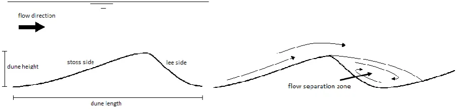
The typical asymmetric form of river dunes is important for the determination of hydraulic roughness of the river bed. Asymmetric dunes generated in a steady, uniform and unidirectional flow induce implications to the flow. Flow resistance, bed shear stress and sediment transport are affected by the shape of these dunes. Turbulence over such dunes is dominated by the flow separation zone and very important for dune formation (Best, 2005). Flow close to the bed follows the bed profile. However, when river dunes have an asymmetric form with steep lee sides, the flow will separate from this profile at the dune crest because the longitudinal flow velocity is larger than the vertical velocity caused by gravitational force. The flow separation results in rotational flow behind the dune crest with variations in the pressure gradient, as presented in figure 1. The rotational flow causes energy loss, a turbulent flow regime and a reverse flow near the bed that result in a zero net discharge through a vertical cross section between the bed and the separation zone (Paarlberg et al., 2007). This leads to a sudden increase in the hydraulic roughness and therefore to an increase of the water level.

FIGURE 1: TYPICAL SHAPE OF A RIVER DUNE (LEFT), PRINCIPLE OF FLOW SEAPARATION (RIGHT)

The influence of river dunes on the river bed and flow is why many have tried and are still trying to model dimensions and propagation of dune models under various circumstances. Understanding the processes that induce dune formation and evolution is key when modelling river dunes. The question is which processes should be included and which should not be included. Assumptions have to be made because models are a simplification of reality and cannot capture all processes.

1.2

S

11

for certain flow conditions. To study the evolution of these dunes, nonlinear feedback mechanisms between flow and bed form amplitude were included (e.g. Ji and Mendoza, 1997; Zhou and Mendoza, 2005). These stability analysis techniques are also applicable in situations that are not in equilibrium. As a result of the improved calculation capacity of computers over the years, numerical codes to simulate dune evolution by solving linked systems of flow, sediment transport and bed morphology were introduced (e.g. Tjerry and Fredsøe, 2005; Giri and Shimizu, 2006). These models enable the prediction of time evolution of dune dimensions, dune shapes and dune migration in a two-dimensional way. Recently Nabi et al. (2013) presented a three-two-dimensional numerical model to simulate morphodynamics in a detailed way. The model provides insight into the physical transport phenomena. Disadvantage of the complex systems mentioned here, is that they are computationally intensive. River bed forms in the field show large dissimilarities over both space and time. Capturing these complex bottom features is still a challenge to researchers and modellers.

Because fast calculations are essential during an upcoming flood event, there is a need for fast model predictions with reliable outcomes. These requirements are not fulfilled by the models that are mentioned before. Their output is limited (e.g. Yalin, 1964; Van Rijn, 1984; Kennedy, 1963; Engelund, 1970; Richards, 1980, Ji and Mendoza, 1997; Zhou and Mendoza, 2005) or models are computationally intensive (e.g. Tjerry and Fredsøe, 2005; Giri and Shimizu, 2006; Nabi et al., 2013). Therefore the focus of this research is on the following two models: the cellular automaton dune model HR Wallingford is experimenting with (Knaapen et al., 2013) and the parameterized dune model of Paarlberg et al. (2009). Both models are relatively fast in their calculations and have a fundamentally different approach to predict river dunes.

Paarlberg et al. (2009) developed a process-based simulation model for river dune evolution that has limited computational effort and therefore is useful for operational water management. They extended the model of Németh et al. (2006) with a parameterization of flow separation (Paarlberg et al. 2007) to enable simulation of finite amplitude river dune evolution. The model is based on hydrostatic flow equations and predicts dune evolution in a two dimensional vertical plane.

HR Wallingford is experimenting with a so called cellular automaton dune model (CA model) to predict dune evolution. CA models are relatively unknown in the world of hydrodynamics, morphology and modelling river dunes. Fonstad (2006) described cellular automata as a class of numerical models based on a discrete space-time grid, each particle in the model is restricted to this grid. Interactions between cells are deterministic, probabilistic or rule based. CA models have been applied for modelling succession on aeolian sand dunes (Baas and Nield, 2010). Murray and Paola (1994) used cellular automata to model river braiding and Werner and Fink (1993) used a cellular automaton type of model to simulate beach cusps as self-organized patterns. Coco and Murray (2007) showed that cellular automata have been used for the simulation of different nearshore patterns. It is further shown that cellular automata are capable of capturing complex patterns of sand waves, ripple and dune formation (Bishop et al., 2002, Nield and Baas, 2008).

12

more simple to initialize, understand and operate in comparison to mathematical deterministic models (Knaapen et al., 2013). In this way, model calculations are relatively short. Therefore this model could also be useful for operational water management. However, length and time scales were not present in the results because output was only presented in number of cells and interactions between cells were based on probabilities. Therefore conclusions on the performance of the model according to dune dimensions, migration rates and time to equilibrium could not be made.

The question for both models remains how accurate they are and what their predictive value is.

1.3

R

The parameterized dune model and the CA model are two models with relatively fast calculations that could be useful for operational water management purposes such as water level predictions during an upcoming flood event. In this research both models are tested under various conditions to assess their performance and provide insight in their strengths and weaknesses. The main objective of this research is:

To compare the performance of the cellular automaton dune model and the parameterized dune model for the prediction of dune dimensions, migration rates and sediment transport in equilibrium state, under flume conditions, similar to low-land river situations like the River Rhine (the Netherlands).

Because the CA model of HR Wallingford is missing essential length and time scales, adjustments are necessary before the model can be compared to data. The model should also be calibrated before the models can be compared. Consequently the following research questions are formulated to serve as a guideline for this research:

1. Which processes are modelled by the parameterized dune model and the

cellular automaton dune model and which input data are necessary to calibrate and validate these models?

2. How to add length and time scales to the cellular automaton dune model and how to relate the input parameters of the model to the data?

3. How well do both models perform compared to flume data?

4. What are the strengths and weaknesses of the parameterized dune model and the cellular automaton dune model?

1.4

T

13

15

C

2

M

ODEL DESCRIPTIONS AND

EXPERIMENTAL DATA

This research starts with a description of the models to gain insight in the modelled processes and input parameters necessary to run these models. The parameterized dune model is analysed using the publications of Paarlberg et al. (2007 and 2009) and by running the model to discover the involved processes. The CA model is analysed by investigating the script and understanding the steps that lead to the output of the model. The publication of Knaapen et al. (2013) supports the understanding of the model and processes involved. Besides, an overview of the experimental data used for the comparison of the model performances is presented. This chapter provides an answer on research question 1.

2.1

T

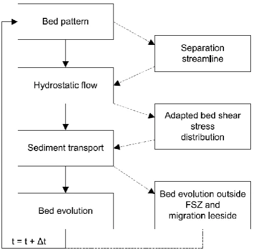
The parameterized dune model used by Paarlberg et al. (2009) is based on the process-based morphodynamic model of Németh et al. (2006). This model is capable to simulate the evolution of dunes under unidirectional flows. Hydrostatic flow equations are the fundamentals of the used flow model, therefore separated flows cannot be analysed. However, Paarlberg et al. (2009) extended the model with a parameterization of flow separation. This parameterization is used to efficiently predict dune dimensions over the timescale of a flood wave instead of using complex hydrodynamic equations. Turbulence over dunes with a lee side angle of repose is dominated by the influence of the flow separation zone (Best, 2005 and references herein). The inclusion of flow separation is essential; without flow separation dunes saturate at an early stage of evolution, resulting in an incorrect dune shape without a slip face and an underestimation of dune height and time to equilibrium (Paarlberg et al., 2007).

16

FIGURE 2: SETUP OF THE PARAMETERIZED DUNE MODEL (AFTER PAARLBERG ET AL., 2009)

2.1.1

P

It is important to know which processes are modelled to compare the predictions of both models in the end. The processes involved in the parameterized dune model are described here.

Flow characteristics

The parameterized dune model is a process-based simulation model for river dune evolution, where flow characteristics are the driving force for sediment transport. The flow field is described by two-dimensional shallow water equations assuming hydrostatic pressure conditions. The essential input parameters can be measured or determined during flume experiments, this makes it straightforward to compare the model with datasets.

Flow separation

Essential for the parameterized dune model is the inclusion of flow separation. The flow is assumed to separate when the bed slope of the dune lee side exceeds a certain threshold. After establishing flow separation, the shape of the flow separation zone is determined. The separation streamline forms a virtual bed over which hydrostatic flow is computed (Paarlberg et al., 2007).

Sediment transport

17

that causes dune evolution is computed using a formula like Meyer-Peter and Müller (1948). Adjustments have been made according to gravitational bed-slope effects and parameter settings. Sediment is transported in the flow direction and deposited along the dune and in the flow separation zone.

Avalanching

In case of flow separation, sediment passing the flow separation point is assumed to avalanche down the leeside of the dune. The sediment will distribute evenly and the leeside slope is assumed constant and equal to the angle of repose for natural sand (30°), which is valid according to Kleinhans (2003). This way the typical asymmetric form of a river dune under unidirectional flow develops.

2.1.2

I

To run the parameterized dune model it is essential to know the bed slope, which is the driving force for the flow. The domain for the simulation is set by two conditions: Water depth to determine the domain height and dune length to determine the domain length. The dune length is determined using a numerical linear stability analysis and is mainly controlled by the initial water depth. From this analysis the fastest growing dune length is found and adopted as domain length. The discharge is used to control the imposed water depth and is defined as the discharge per second per meter width. The initial water depth is used to help the model with a first estimation of the water depth. This will speed up the process at the start. The grain size is essential for calculation of the sediment transport.

Model parameters to check are the parameters defining the characteristics of the fluid, the characteristics of the sediment and the gravitational acceleration. The density of water needs to be set for the calculation of the influence of the characteristics of the fluid. The characteristics of the sediment are defined by the density of sediment, porosity and the angle of repose. Besides, the critical shields parameter is assumed to be constant as this was also adopted by Paarlberg et al (2009).

2.1.3

O

18

2.2

T

The CA model of HR Wallingford is based on the study of Bishop et al. (2002). It is a model operating in a discrete three-dimensional space and simulating changes to the bottom profile. The model consists of a three-dimensional lattice that can be considered as a grid of stacked slabs. Sediment transport is simulated by the interaction between cells in the grid. Interactions are based on a stochastic set of rules that determine the chance on different events. Initially the model only focuses on uniform sediment, while Knaapen et al. (2013) modify the basic CA model by adding multiple grain types. In this way it becomes possible to model the principle of larger particles covering smaller particles and the sortation of sediment particles over bed forms. The critical difference between a model with specific grain types and the basic model is that each slab in the model needs to be identified and tracked which requires much more memory capacity.

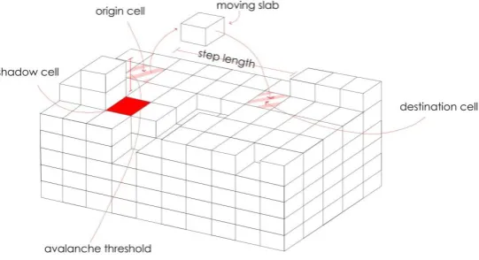
The basic rules of the CA model are depicted in figure 6. First a cell is picked at random where the top slab is selected; a pickup probability distribution determines whether the slab will be picked up. When the selected slab is in shadow the chance to be picked is nil and another cell will be selected. A slab that will be picked up is shifted forward in the predefined direction of the current. The moved slab is deposited on top of the stack of slabs at the destination cell. At this cell it may ‘stick’ and remain there or ‘bounce’ and move again, which simulates the principle of saltation. When the slab sticks, a process of local avalanching is initiated. This process is also triggered at the origin cell when a slab is picked up. After this process a new cell is randomly selected, this process is repeated for a preset amount of slots. The amount of slots represents the number of random cell selections (‘pick a random cell’ in figure 6).

The model is based on stochastic rules, there is no direct relation to flow characteristics like flow velocity, water depth or slope. Dimensions are not defined in the model, only the amount of cells can be defined and probabilities according to the sediment distribution. Thus the model has no input parameters that could be compared to the data set or parameterized dune model. Therefore adjustments have to be made to provide the CA model with length and time scales.

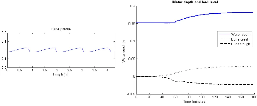
FIGURE 3: DUNE PROFILE OF FOUR IDENTICAL DUNES AS PREDICTED BY THE PARAMETERIZED DUNE MODEL, FLOW DIRECTION FROM LEFT TO RIGHT

19

FIGURE 5: SCHEMATIC OVERVIEW OF THE PROCESSES INVOLVED IN THE CELLULAR AUTOMATON DUNE MODEL

20

2.2.1

P

It is important to know which processes are modelled to compare the predictions of both models in the end. The processes involved in the CA model are described here.

Sediment transport

The model solely exists of sediment that forms the river bed or sediment that is moving in a predefined direction; the direction of the flow. Flow conditions, as incorporated in the parameterized dune model, are not present in the CA model. The simulated sediment transport concerns only bed load transport, suspended sediment is neglected. Sediment transport is simulated by moving slabs in the flow direction and depositing them on top of other slabs.

Shadow zone

The shadow zone reflects the areas in a flow where velocities are negligible and sediment will always be deposited, comparable with the flow separation zone of the parameterized dune model. A cell is picked at random where the top slab is selected, if the slab is in shadow it does not move, if it is not in shadow the slab is shifted forward in the direction of the current. When a destination cell is in shadow, the slab will always stick.

Saltation

A moved slab is deposited on top of the stack of slabs at the destination cell. At this cell it may ‘stick’ and remain there or ‘bounce’ and move again. This process is also observed in nature, where sediment particles in bed load transport touch the ground and move on before they deposit.

Avalanching

When a slab sticks on a destination cell a process of local avalanching is initiated. Avalanching involves a move to a neighbouring cell if the slope of the stack of slabs in that direction exceeds the angle of repose. Fill back is the opposite of this process that might occur when a slab is moved and the slope at the origin cell may exceed the angle of repose, this also causes avalanching.

Sediment sorting

The CA model is capable of capturing the sorting process of sediment due to different grain sizes. The grain size distribution is used to link sediment characteristics to probabilities; this reflects the sediment behaviour in real rivers (Blom et al., 2003). This process cannot be simulated by the parameterized dune model and is not included in this research.

2.2.2

I

21

These shear velocity constants are indirectly related to the shape of the flow profile. The grain size distribution of the sediment enables one to add different grain sizes, their characteristics can be set by changing the pickup and deposition probability.

Model parameters to check are the number of cells in each direction to establish the grid, sediment characteristics and model characteristics. The angle of repose determines the difference in number of slabs between neighbours before an avalanche is triggered. The shadow distance determines how far to search for shadow zones. Also the number of slots have to be set once, this is the amount of slabs that will be selected during a model run.

2.2.3

O

The main output of the CA model is the evolution of the bed in a three-dimensional way. Bed formations can be presented restricted to differences in number of cells only. Dune dimensions can be counted in number of cells. There is no relation with length or time scales so migration rate and sediment transport are not present. Adjustments have to be made before comparing the model with the parameterized dune model or experimental data.

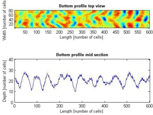
In contrast to the parameterized dune model, the CA model shows a field of dunes that varies in height and length over the domain. A bottom profile predicted by the model is presented in figure 7. The mid section of the bed profile shows variations in dune height, length and shape of the dunes. The driving force for sediment transport in the CA model is the step length. Although output seems promising, results cannot be compared with field observations in a quantitative manner. This is due to the absence of length and time scales. The question is how to adjust the CA model in a way it can be compared with flume experiments and the parameterized dune model?

22

2.3

O

The difference in approach of modelling is reflected in the modelled processes and input parameters required to run both models. Overviews are presented and discussed in this section.

2.3.1

M

An overview of the modelled processes is presented in table 1 to gain insight in the similarities and dissimilarities of the model approaches.

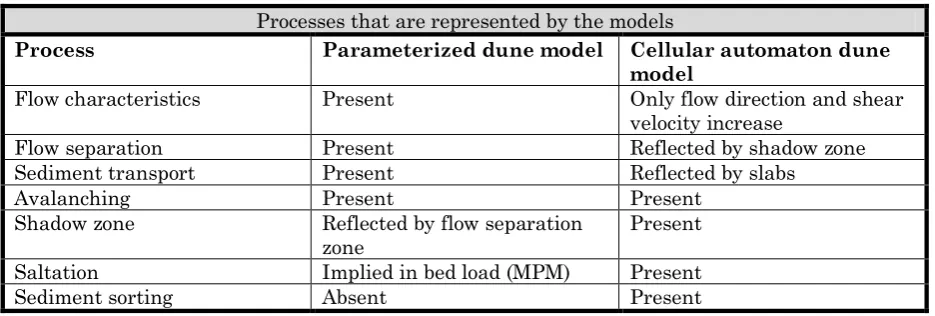
TABLE 1: PROCESSES MODELLED BY EACH MODEL

Processes that are represented by the models

Process Parameterized dune model Cellular automaton dune

model

Flow characteristics Present Only flow direction and shear velocity increase

Flow separation Present Reflected by shadow zone Sediment transport Present Reflected by slabs

Avalanching Present Present Shadow zone Reflected by flow separation

zone Present Saltation Implied in bed load (MPM) Present Sediment sorting Absent Present

Predictions of the parameterized dune model are based on the flow characteristics, whereas in the CA model only flow direction and shear velocity increase are included to determine the shape of the flow profile. Sediment transport is simulated in two different ways. The parameterized dune model uses a sediment transport formula to calculate the dune development, while the sediment transport in the CA model is represented by moving slabs of sediment based on stochastic rules. The process of saltation is explicitly incorporated in the CA model, whereas in the parameterized dune model it is implied by bed load transport. The presented overview of processes is useful for the comparison of both models to declare the differences in outcomes.

2.3.2

I

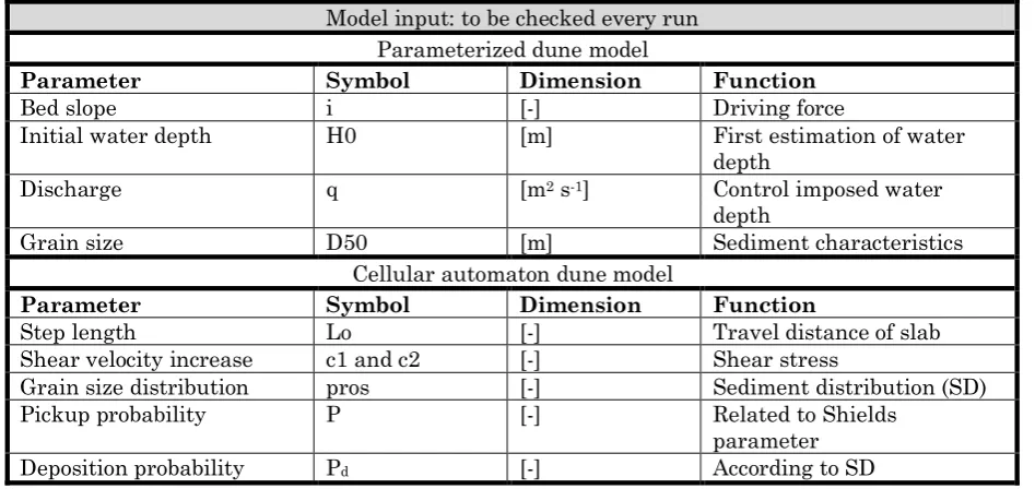
Overviews of the model input and parameters are presented in tables 2 and 3 that serve as guideline to select appropriate data sets.

Model input

23 TABLE 2: MODEL INPUT FOR EACH MODEL

Model input: to be checked every run Parameterized dune model

Parameter Symbol Dimension Function

Bed slope i [-] Driving force

Initial water depth H0 [m] First estimation of water depth

Discharge q [m2 _s-1_{] Control imposed water}

depth

Grain size D50 [m] Sediment characteristics Cellular automaton dune model

Parameter Symbol Dimension Function

Step length Lo [-] Travel distance of slab Shear velocity increase c1 and c2 [-] Shear stress

Grain size distribution pros [-] Sediment distribution (SD) Pickup probability P [-] Related to Shields

parameter Deposition probability Pd [-] According to SD

Model parameters

Besides the model input that depend on the experiments and have to be checked each run, the models also include parameters that are independent of the experiments and therefore should be checked before starting the validation phase.

TABLE 3: MODEL PARAMETERS FOR EACH MODEL

Model parameters: to be checked once Parameterized dune model

Parameter Symbol Dimension Function

Density of water ρw [kg m-3] Water characteristics

Density of sediment ρs [kg m-3] Sediment characteristics

Porosity εp [-] Sediment characteristics

Angle of repose θrepose [°] Sediment characteristics

Gravitational acceleration G [m s-2_{] Acceleration due to gravity}

Critical shields parameter θcr [-] Critical shear stress

Cellular automaton dune model

Parameter Symbol Dimension Function

Number of cells xlen, ylen and zlen [-] Grid dimensions

Angle of repose Rep [-] Avalanche trigger Shadow distance sDist [-] Distance to search for

shadows Shadow angle sAng [-] Shadow zone

Number of slots Slot [-] Amount of selected slabs

24

2.4

D

The focus of this research is on river dunes which are dominant in low-land rivers with a sandy bed such as the River Rhine (the Netherlands). Therefore, conditions of the experiments should be comparable to this type of rivers. Flow in this type of rivers is always subcritical (Fr << 1)1_{. Under subcritical flow conditions bed load transport is}

dominant. The influence of suspended sediment transport can be safely neglected when Froude numbers are small (Fr < 0.5) (Paarlberg et al., 2009). The selected data have to contain the required input parameters described in section 2.3. However, not only input values are important in this research, because model output of dune dimensions and migration rates will be compared. Also the flume experiments have to show the values of dune height, dune length and migration rates to compare the model predictions with measures of the flume experiments. Data of flume experiments requires the information presented in table 4. A variety of circumstances is selected, resulting in a dataset containing 17 experiments; a single experiment for calibration and 16 experiments for validation.

TABLE 4: PARAMETERS WHERE DATA SELECTION IS BASED ON

Input Output Bed slope Measured dune height Water depth Measured dune length Discharge Measured migration speed Grain size

2.4.1

D

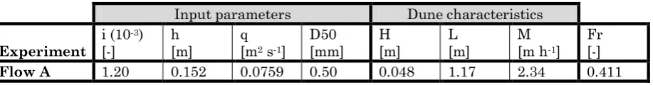
To ensure that the comparison of model results is based on the same conditions, both models should be calibrated using the same data. The parameterized dune model is already calibrated. Paarlberg et al. (2009) calibrated the model using flow A as reported by Venditti (2003). The value of each parameter and the results according to flow A are presented in table 5. These values are also used to calibrate the CA model.

TABLE 5: DATA USED FOR CALIBRATION (AFTER VENDITTI, 2003)

Input parameters Dune characteristics

Experiment i (10

-3₎

[-] h [m] q [m2 _s-1_]

D50

[mm] H [m] L [m] M [m h-1_]

Fr [-]

Flow A 1.20 0.152 0.0759 0.50 0.048 1.17 2.34 0.411

2.4.2

D

The data set used for the validation phase is a small selection of the data set used by Naqshband et al. (2014). The final data set used for validation contains sixteen experiments, consisting of four equal sets of four experiments. The first selection is based on four experiments of Venditti (2003) partly used by Paarlberg et al. (2009) as well, although input and output values are used slightly different in the research of

25

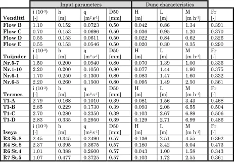
Paarlberg et al. (2009). The expectation is that predictions of the models are closest to the observed characteristics for these experiments. As circumstances of these experiments are close to conditions of flow A that is used for calibration. The data have a varying Froude number and a constant median grain size of 0.5 mm. The second set used for validation is data set II: Fixed layer experiments large flume (DS-II) of Tuijnder (2010). Although the main purpose of the research is on supply limited conditions, six experiments were executed without a limitation in sediment supply (alluvial conditions). The validation on data of Tuijnder (2010) will be based on four experiments with a varying Froude number, comparable to the data of Venditti (2003) and a larger median grain size of 0.8 mm to discover the effects of a changing grain size. The third set used is the data set of the flume experiments of Termes (1986). The validation on data of Termes (1986) will be based on four experiments with slightly higher Froude numbers in comparison to the data of Tuijnder (2010) and Venditti (2003) and a smaller median grain size of 0.39 mm. The last set used is derived from case 2 of the flume experiments of Iseya (1984). The data set of Iseya (1984) contains four experiments with a combination of two different discharges and two different slopes. The experiments were conducted in a larger flume compared to the other experiments; however Froude number and grain size are comparable to the data of Venditti (2003). Table 6 represents the data of Venditti (2003), Tuijnder (2010), Termes (1986) and Iseya (1984) that will be used for the validation phase. Additional information about the experimental conditions and measurement methods can be found in appendix A.

TABLE 6: DATA USED FOR VALIDATION (AFTER VENDITTI, 2003; TUIJNDER, 2010; TERMES, 1986 AND ISEYA, 1984)

Input parameters Dune characteristics

Venditti i (10

-3₎

[-] h [m] q [m2 _s-1_]

D50

[mm] H [m] L [m] M [m h-1_]

Fr [-]

Flow B 1.10 0.152 0.0723 0.50 0.042 0.86 1.34 0.391

Flow C 0.70 0.153 0.0696 0.50 0.036 0.95 1.20 0.370

Flow D 0.55 0.153 0.0611 0.50 0.022 0.84 0.62 0.326

Flow E 0.55 0.153 0.0546 0.50 0.020 0.30 0.35 0.290

Tuijnder i (10

-3₎

[-] h [m] q [m2 _s-1_]

D50

[mm] H [m] L [m] M [m h-1_]

Fr [-]

Nr.5-7 1.50 0.200 0.0940 0.80 0.070 1.39 1.00 0.336

Nr.1-10 2.20 0.200 0.1050 0.80 0.077 1.44 1.90 0.375

Nr.6-1 1.70 0.250 0.1300 0.80 0.083 1.47 1.60 0.332

Nr.6-3 2.20 0.260 0.1500 0.80 0.095 1.49 2.50 0.361

Termes i (10

-3₎

[-] h [m] q [m2 _s-1_]

D50

[mm] H [m] L [m] M [m h-1_]

Fr [-]

T1-A 2.79 0.168 0.1010 0.39 0.081 1.56 3.43 0.468

T1-B 2.85 0.229 0.1730 0.39 0.093 2.08 6.55 0.504

T1-C 2.70 0.280 0.2350 0.39 0.103 2.67 6.89 0.506

T1-D 2.83 0.335 0.2950 0.39 0.129 2.71 6.99 0.486

Iseya i (10

-3₎

[-] h [m] q [m2 _s-1_]

D50

[mm] H [m] L [m] M [m h-1_]

Fr [-]

R3 St.8 2.45 0.345 0.2490 0.57 0.136 2.51 4.55 0.392

R4 St.8 2.37 0.395 0.3675 0.57 0.180 3.42 5.04 0.473

R6 St.4 1.01 0.388 0.2600 0.57 0.043 1.00 1.58 0.343

26

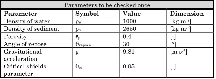
Besides the data selection for validation, all fixed parameters as discussed in section 2.3 need a value before starting with the model runs. As mentioned earlier, it is assumed they will be constant and will not change during the model runs. The density of water and sediment are assumed to be common used values, respectively 1000 kg m-3 _{and 2650}

kg m-3_{. The porosity of the sediment is assumed to be 40%, this is also the default value}

for porosity in the parameterized dune model. The angle of repose is set for the characteristic value of sand which is 30°. The gravitational acceleration parameter g is set on 9,81 m s-2_{. An overview of these parameters is provided in table 7.}

TABLE 7: VALUES FIXED PARAMETERS

Parameters to be checked once

Parameter Symbol Value Dimension

Density of water ρw 1000 [kg m-3]

Density of sediment ρs 2650 [kg m-3]

Porosity εp 0.4 [-]

Angle of repose θrepose 30 [°]

Gravitational

acceleration g 9.81 [m s

-2_]

Critical shields

parameter θ

27

C

3

R

ESEARCH METHODOLOGY

This research consists of two steps to reach the final goal. Each step is described in a separate chapter. The first step is the preparation of the CA model for the validation phase. To do so, a sensitivity analysis reveals the behaviour of the model, length and time scales are added to the model and the input parameters of the model are linked to the flow characteristics. The CA model is calibrated after these adjustments. Research question 2 is answered by finishing the first step. The second step is the comparison of the parameterized dune model and the CA model with the prepared data sets. Output of the models is analysed and both models are discussed which leads to the answers on research questions 3 and 4. The used methods are described in this chapter.

3.1

A

The initial CA model is based on stochastic rules; there is no link between sediment transport and flow characteristics within the model. It is not possible to relate experimental data to the model without making adjustments to the model.

3.1.1

S

28

3.1.2

P

The CA model is adapted before the model is calibrated. The model has not been used for dune evolution predictions under flume conditions before. Therefore adjustments to the model are made before comparing it with the parameterized dune model. A length scale is added by linking the model parameters to a distance instead of a number of cells and assuming a fixed domain. In this way parameters and the domain itself are defined in meters and no longer in number of cells. The moved sediment within the model is determined by counting the number of slabs and the distance travelled. The amount of moved sediment is used to add a time scale to the model by relating it to the sediment transport according to Meyer-Peter and Müller (1948). Additionally model parameters of the CA model are linked to the characteristics of the experimental data by using theories to relate flow characteristics with input parameters of the CA model. The adjustments lead to new input parameters for the model; these are the step length, pickup probability, shadow distance and sediment transport.

3.1.3

C

After the CA model is adjusted it needs to be calibrated before the actual comparison with the parameterized dune model. Predictions are compared to the observed data of experiment flow A (Venditti, 2003). Differences between the model output and the observed data are minimized by adjusting model parameters. The parameters not defined by input characteristics are used for the calibration of the CA model; these are the amount of cells, shear stress velocity and run time of the model. The sensitivity analysis provides insight in the behaviour of those parameters and therefore facilitates the calibration process. Because of the long runtime of the CA model, calibration is done manually by trial and error. The model is calibrated by running the model and changing each calibration parameter separately for a wide range (± 25-400%). The best approximations are combined and small changes in the parameters are tested to further improve the predictions of the model (± 1-10%).

The dimensions are determined using the bedform tracking tool of van der Mark et al. (2008). The average of three sections parallel to the flow direction determines the dimensions. Transects are selected at the first quarter, midsection and third quarter of the domain. Dune height is defined as the distance between the top of a crest and the consecutive downstream trough. Dune length is defined as the distance between two consecutive troughs. The migration rates are determined by selecting five dune troughs at random and compare the output of the final result with the result of 19/20 of the total runtime. The mean difference between the troughs is assumed to be the displacement of the dunes. The time is known; therefore the migration rate can be determined for each experiment.

FIGURE 8: DETERMINATION OF DUNE DIMENSIONS FIGURE 9: DETERMINATION OF THE MIGRATION

29

3.2

C

The performance of the parameterized dune model and the CA model is tested using sixteen experiments (as described in chapter 2) to determine their predictive value for prediction of dune dimensions and migration rates. An overview of the input parameters can be found in appendix B (table A). The focus of the validation phase is on the performance of both models compared to the experimental results. The first runs are performed using the data of Venditti (2003) to examine the performance of both models under conditions close to the calibration experiment. Runs for data of Tuijnder (2010), Termes (1986) and Iseya (1984) are performed to examine the models for conditions with various grain sizes, Froude numbers and flume widths.

The output of the parameterized dune model is generated by running the model until equilibrium state is reached. The time to run a single experiment varied between 50 minutes and 3.5 hour. There is no equilibrium state in the CA model, therefore runtime of the model is used as a calibration parameter and assumed to be independent of the input parameters during the validation phase. Runtime of the CA model varied between 10 minutes and 25 minutes. Dune height and length for the predictions of the CA model were provided using the bedform tracking tool of van der Mark et al. (2008) and migration rates are determined by selecting five dune troughs at random and determining the displacement, as described in section 3.1.3.

31

C

4

A

DJUSTMENTS OF THE CELLULAR

AUTOMATON DUNE MODEL

4.1

S

Default settings of the model are presented in table 8. A bottom profile with dunes develops under these conditions as visible in figure 10. This situation is the initial condition that is used in this sensitivity analysis.

TABLE 8: DEFAULT SETTINGS CA MODEL

Default settings

Parameter Value

Slots (number of cells) 50.000 Cells x-direction 10 Cells y-direction 500 Cells z-direction 200 Step length (Lo, number of cells) 12 Linear shear velocity

parameter (c1) 0.3 Non-linear shear velocity

parameter (c2) 0.004 Shadow distance (sDist,

number of cells) 5

Slots

Changing the amount of slots influences the dimensions of the resulting dunes. When the number of slots is set too low, no regular bedform patterns form (top view figures 11 and 12). The bottom profile shows only random patterns, this is likely to be the result of a lack in sediment transport. Increasing the number of slots leads to patterns that start to look like dunes (second view figures 11 and 12). Further increase of slots leads to a regular pattern of bedforms (third view figures 11 and 12). The larger the number of slots, the longer, higher and more asymmetrical the dunes will grow and thus, the number of dunes in the domain will decrease (last view figures 11 and 12). An extremely long run is presented; dunes are merged into a large dune and three smaller dunes. A further increase of slots will finally result in a single dune that covers the whole domain. This is a problem within the model because dunes keep growing; an equilibrium state is not reached.

32

TABLE 9: RESULTS SENSITIVITY ANALYSIS SLOTS

Sensitivity analysis slots

Figures

11 and 12 Slots (*103₎

Dunes Height

A 12.5 - - B 37.5 ± 9 ± 12 C 100 8 ± 40 D 5000 4 ± 75

Grid cells

Changing the number of grid cells shows that dune formations are directly related to the grid size. Doubling the number of cells in z-direction (height of the domain) does not affect the amount of cells within the dune. Changing the number of cells in the direction of the flow (y-direction) shows the same relation, the amount of cells in a single dune does not change. More dunes will develop in the fixed domain with a larger amount of cells in y-direction. Thus dune dimensions depend on the grid size, assuming that the domain has dimensions; however this should not be the case.

TABLE 10: RESULTS SENSITIVITY ANALYSIS GRID CELLS

Sensitivity analysis grid cells

z-direction y-direction

Cells in

z-direction Dunes in domain Height in cells Cells in y-direction Dunes in domain Height in cells 100 8 ± 40 250 5 ± 40 200 8 ± 40 500 8 ± 40 300 8 ± 40 750 11 ± 40

FIGURE 11: TOP VIEW BOTTOM PROFILE CHANGING SLOTS, (IN ORDER 12.5, 37.5, 100 AND 5000 (*10^3)) VALUES ON AXIS IN NUMBER OF CELLS, FLOW DIRECTION FROM LEFT TO RIGHT

33

Step length

Changing the step length shows a relation between dune length and step length, although there are some transition zones. In general, an increasing step length leads to an increase in dune length; fewer dunes will develop. Between step lengths of 20 to 25 cells something strange happens, the developed patterns become irregular. After increasing the step length further, regular patterns are formed again with an increase in number of dunes and thus a decreasing dune length. Further increase of the step length leads to a further decrease of number of dunes, until a new transition zone is reached (around a step length of 60). It seems that dunes developed at larger step lengths show more constant forms with less variations than dunes developed at smaller step lengths. There is no observed relation between step length and dune height.

TABLE 11: RESULTS SENSITIVITY ANALYSIS STEP LENGTH

Shear velocity

Changing the linear shear stress component (c1) has influence on the dune height. Decreasing the component leads to an increasing dune height, while increasing the component leads to a decreasing dune height. Dune length is not influenced by changing the component, although the form seems to be more asymmetric when the component is getting lower. Changing the non-linear component (c2) results in a change in dune form; with a decreasing non-linear component, dunes develop more asymmetrically with steeper lee sides and stoss sides that are more flattened. Also dune height is affected by changes; decreasing the component leads to an increase in dune height. Both components show similar behaviour according to dune form and dimensions, although the first component seems to have more effect on the dune height, while the second component has the largest influence on the asymmetrical shape of the dune.

Sensitivity analysis step length

Figure

13 Step length Dunes Height

A 8 10 ± 20 B 15 7 ± 21 C 20 - - D 40 14 ± 19 E 50 11 ± 21 F 60 17 ± 21

34

TABLE 12: RESULTS SENSITIVITY ANALYSIS SHEAR VELOCITY

Shadow distance

Shadow distance is tested under various conditions. Changing the shadow distance seems to have almost no influence on the dune dimensions. Number of dunes and dune height remain approximately the same. It is important to ensure this parameter is set large enough to search for the former dune crest.

Conclusions

The sensitivity analysis provides insight in the behaviour of the input parameters. Relations between individual cells according to angle of repose, step length, shadow distance and so on are all based on a number of cells. Increasing the number of cells leads to decreasing dune dimensions. It is important to separate this relation in a way that the amount of grid cells determines the level of detail of the dune instead of the number of dunes in the domain. The step length can be seen as the driving force for sediment transport in the CA model. In reality flow velocity is responsible for sediment transport. This parameter should be linked to the flow velocity of the experimental data to make comparison of both models and the data possible. The shear velocity is important for the fine tuning of the model and can be an important parameter for the calibration process.

Sensitivity analysis shear velocity

Fig. 14 c1 c2 Dunes Height

A 0.3 0.004 7 ± 50 B 0.2 0.004 7 ± 70 C 0.4 0.004 7 ± 25 D 0.3 0.003 7 ± 52 E 0.3 0.005 7 ± 48

35

4.2

P

A length scale is added to the CA model by linking the model parameters to a distance instead of a number of cells and assuming a fixed domain. The sediment transport within the model is determined and a time scale is added. Additionally model parameters of the CA model are linked to the characteristics of the experimental data.

4.2.1

L

The first step to add a length scale to the CA model is assuming a fixed domain and defining the dimensions of that domain. In this way increasing the number of cells lead to a more detailed grid with smaller cells, while the domain dimensions remain the same. The predefined domain is divided into the number of determined cells, where each cell has dimensions of:

, ( 1 )

, ( 2 )

, ( 3 )

where dx, dy, dz is the length of one cell in x-, y- or z-direction, Lx, Ly, Lz is the length of the domain in the corresponding direction and nx, ny, nz is the number of cells in the corresponding direction. In this way the dimensions of the domain are fixed and the dimensions of a single cell can be determined. Each cell has the same dimensions; therefore distances and thus dune dimensions can be easily determined. Also the volume of sediment transported within the model can be calculated. The next step is relating the model parameters to a distance instead of a number of cells. The parameters are adjusted to create model parameters defined in a length scale.

Angle of repose

The angle of repose in the CA model was defined as a number of slabs in z-direction. When the slab difference between neighbours exceeds this amount of slabs, an avalanche is triggered. Adjusting this parameter to link the amount of slabs to the angle of repose is necessary. To do so, the dimensions of each cell in both height (z-direction) and length (y-direction) are used. The ratio between these dimensions determines the amount of slabs (Rep) in the z-direction needed to create the angle of repose ( ). In formula:

. ( 4 )

36

Step length

The step length in the CA model was defined as a number of slabs. Increasing the number of cells in the domain leads to a decrease in step length. The step length is linked to the grid to overcome this problem. Step length defined in cells (Lo) is determined as follows:

, ( 5 )

where Lo’ is the parameter that defines the step length in meters and dy is the length of a single cell in the flow direction. The result needs to be an integer, because the model only counts cells. Therefore the closest number of cells is selected which leads to an approximation of the step length that varies between 3 and 18 cells for this research.

Shadow distance

The shadow distance was also defined as a number of slabs to search for the shadow zone. Thus the problem for the step length also applied for shadow distance. The shadow distance defined in cells (sDist) is linked to the grid in the following way:

, ( 6 )

where sDist’ is the parameter that defines the shadow distance in meters and dy is the length of one cell in the flow direction. The result needs to be an integer, because the model only counts cells. Therefore the closest number of cells is selected which leads to an approximation of the shadow distance that varies between 4 and 35 cells for this research.

Slots

The number of slots determines how many cells will be selected each model run. This number is set in a way that the amount of sediment that could be transported is the same for each run. Therefore the number of slots is chosen in a way that it is a multiplicity of the number of cells on the surface:

, ( 7 )

where slotp is the slot parameter that determines how many times the total surface will be selected each run and nx and ny are the number of cells in x- and y-direction respectively.

37

4.2.2

T

A time scale is added to the CA model by using the sediment transport for both the model and the experiments. The sediment transport of the experiments is determined using the sediment transport formula of Meyer-Peter and Müller (1948) with a correction according to Wong & Parker (2006). The value for the empirical coefficient m is 4 instead of 8 and the critical Shields number θcr is 0.05 instead of 0.047 as proposed

by Meyer-Peter and Müller (1948). These values are also used for the parameterized dune model (Paarlberg et al. 2009). The initial sediment transport is calculated using the data of the experiments and the corrected formula of Meyer-Peter Müller (1948). The sediment transport is determined using the following equations.

, ( 8 )

where is the non-dimensional transport parameter and the non-dimensional flow parameter defined in the following way:

, ( 9 )

, ( 10 )

where qs is the sediment transport volume of solid material per unit width. This is the

volume without porosity; the initial sediment transport is adjusted to include the porosity. The acceleration due to gravity is denoted by g and Δ is the mass of sediment minus the mass of water divided by the mass of water ((ρs – ρw) / ρw). D is the grain

diameter of the sediment; C denotes the Chézy coefficient and C90 is related to D90 in the

following way:

. ( 11 )

The transported sediment in the model is determined by using the total step length of all moved slabs and multiplying the result with the volume of one cell. This leads to the total distance travelled by a single slab, dividing this by the domain length will result in the total amount of sediment transported. In formula:

, ( 12 )

where ST is the total sediment transport per unit width, Slt is the total step length of all the moved slabs in number of cells, dy is the length of an individual cell in meters, vol is the volume of one cell in m3_{, Lx is the length of the domain in the x-direction in meter}

and Ly is the length of the domain in y-direction in meter.

38

determined by dividing the total transport in the model (ST) by the sediment transport (qs) including the porosity (εp), in formula:

, ( 13 )

In this way a time scale is added and migration rates and time to equilibrium of dunes can be predicted. Together with the dune dimensions, these are the most important characteristics to compare, because they influence the roughness and changes to the riverbed.

A disadvantage of the presented method is that sediment transport in the model is assumed to be equal to the calculated sediment transport according to the sediment transport formula. In other words, the sediment transport in the CA model is based on measurements during the experiments instead of a modelled sediment transport. In this way it is impossible to compare predicted sediment transport rates of both models with the data, because the sediment transport rate in the CA model will be exactly the same as the outcome of the sediment transport formula.

4.2.3

L

After implementing time and length scales to the CA model, it is possible to link the model to the experimental data. Pickup probability, deposition probability, step length and shadow distance are related to the results of the experiments. To do so, a couple of assumptions are made. The used methods and theories to link the input parameters to the experimental data are described here.

Pickup probability

The pickup probability in the CA model is a measure for the ability of the sediment to be set in motion. This pickup probability depends on the grain size of the sediment and the flow characteristics such as flow velocity. To link the pickup probability to the circumstances of the experiments there should be a relation between the sediment, flow characteristics and pickup probability.

Cheng & Chiew (1998) proposed a method to relate the pickup probability with the shields parameter, a measure for the initiation of motion of sediment in a fluid flow. They based their formula on earlier studies of Engelund and Fredsoe (1976) and Fredsoe and Deigaard (1992).

, ( 14 )

where θ is the shields parameter, the dimensionless shear stress and CL denotes a

39

The CA model is linked to the flow circumstances and grain size of the sediment by using this formula. Important to mention is that the method of Cheng & Chiew (1998) is designed for single sediment particles and the CA model is calculating with slabs of sediment. This method only holds, when the assumption is made that the behaviour of single particles and the slabs in the model are the same. Further research on the application of this method is necessary to determine whether this assumption is reliable or not.

Deposition probability

Besides the pickup probability as described above, there is also a deposition probability in the CA model. Heavier particles and lower flow velocities result in lower values of the shields parameter and therefore a lower pickup probability. This principle should also be reflected in the deposition probability. Therefore it is assumed that the deposition probability is denoted as:

, ( 15 )

where Pd is the deposition probability and P is the pickup probability.

Step length

Flow velocity is an important parameter in dune evolution and affects dune dimensions. The travel distance of sediment in transport is influenced by the flow velocity. No flow velocity is present in the CA model; however the step length determines the travel distance of the slabs. Therefore these two parameters should be linked in a way to represent the flow velocity in the CA model.

Sekine & Kikkawa (1992) proposed a relation between the shear and settling velocity and the step length of saltating grains. The shear and settling velocity can be derived from the experiments and the step length of saltating grains is included in the CA model as step length of slabs. The resulting relation is denoted by the following formula:

, ( 16 )

where λ is the dimensionless step length, α2 is a constant with value 3.0*103, u* is the

shear velocity [m s-1_{], vs denotes the settling velocity of the sediment [m s}-1_{] and u*c is the}

critical shear velocity [m s-1_{]. The dimensionless step length is related to the step length}

in [m] in the following way:

, ( 17 )

where Λ is the step length in [m] and D the grain size in [m].