and
Shape Reconstruction
A thesis presented for the degree of Doctor of Philosophy
in Electrical & Electronic Engineering at the
University of Canterbury, Christchurch, New Zealand.
by
Ross David Murch B. E. (Hans 1)
' I l
-l
1
cro
Abstract
Investigations of new and improved solutions to inverse problems are considered. Three of the solutions are concerned with inverse scattering. The other two solutions deal with reconstructing binary images from few projections and determining the shape and orientation of a three-dimensional object from silhouettes. In addition, a review of solutions to direct and inverse scattering problems is presented.
An inverse scattering algorithm for reconstructing variable refractive index distri-butions is examined. The inversion algorithm is based on an expression for the wave function which explicitly incorporates the inverse scattering data. It is claimed that this considerably increases the efficiency of the algorithm. The algorithm is implemented in two-dimensional space and examples of reconstructions of objects from computer-generated scattering data are presented.
The problem of determining the shape of a two-dimensional impenetrable obstacle from a set of measurements of its far-field scattering amplitude is considered. The problem is formulated as a non-linear operator equation which is solved by an iter-ative method. The use of the null-field method to solve the direct problem leads to efficient evaluation of the Fnkhet derivative of the non-linear operator. Computational implementations confirm the numerical accuracy of the algorithm.
An extension to the Rayleigh-Gans (Born) approximation is examined. The exten-sion involves incorporating a high frequency approximation to the wave field into the conventional Rayleigh-Gans (Born) approximation. Numerical implementation of an algorithm based on this extension to the Rayleigh-Gans (Born) approximation indi-cates that its reconstruction accuracy is generally superior to that of the conventional Rayleigh-Gans (Born) approximation.
Efficient algorithms for reconstructing a binary cross-sec~ion (each of whose pixel amplitudes is either zero or unity) from few one-dimensional projections are introduced and illustrated by example. It is shown that only two projections are needed to recon-struct a convex cross-section. Non-convex cross-sections need more projections but far fewer than are necessary to reconstruct grey-scale images. When presented with noisy one-dimensional projections, the algorithms remain useful, although their performance improves with the number of given projections.
Determination of a three-dimensional object's shape and orientation from its sil-houettes is studied, on the understanding that the relative orientations of the given silhouettes are unknown a priori. The result of this study is an algorithm which could be suitable for incorporation into a robot's vision system. The algorithm is based on a method for determining the orientation of an object from its two-dimensional projec-tions. To overcome the reduced information content of silhouettes as compared with two-dimensional projections, a self consistency check is introduced. Numerical imple-mentations of the algorithm confirm that it can generate usefully accurate estimates of the orientations and shapes of technologically non-trivial objects.
I wish to sincerely thank my supervisor, Professor R. H. T. Bates, for his enthusiasm, inspiration and persistence. I have benefited greatly both academically and personally from his supervision, and am truly indebted to him.
Collaborators Dr T. John Connolly, Dr Susanne M. Dale, S. Tony Enright, Bruce P. McGregor, Vaughan A. Smith, Dr David G. H. Tan and Dr David J. N. Wall have also been invaluable. Their expertise and imagination have generated excitement in my research. The past and present members of Room 7, my study room, are also thanked for their friendliness and honesty. I also express gratitude to the people studying and working around me as they have provided support and creative discussions. The generous financial help given by Telecom corporation of New Zealand has also been much appreciated.
I especially thank my family and friends for always being there to lean on. Of particular mention is Dr Alan Murch, my brother, whose rare perspective on life has always enlightened me. Andrea McBride and Bruce McGregor, two very special and dependable friends, have also made my studies very memorable. Their distracting influence has kept me sane, I think!
Abstract
Acknowledgements
Preface
1 Introduction
1.1 Review of Practical Inverse Methods . . . . 1.1.1 Seismic Methods in Geophysics . . . . . 1.1.2 Ultrasonic Methods in Medical Imaging 1.1.3 Computed Tomography . . . . 1.2 Research Directions for Practical Inverse Methods
1.2.1 Seismic Methods in Geophysics . . . 1.2.2 Ultrasonic Methods in Medical Imaging 1.2.3 Computed Tomography . .
1.3 Archetypal Problems . . . . 1.3.1 Terminology and Notation. 1.3.2 The Direct Problem . 1.3.3 The Inverse Problem . . . . 1.4 Solving the Inverse Problem . . . .
1.5 Impact of Dimensionality of Space on Inverse Problems
2 Mathematical Preliminaries
2.1 Mathematical Models of the Physics of Scattering. 2.1.1 Time Domain Formulations . . . .
iii v xi 1 1 2 4 5 8 8 9 9 10 10 12 12 13 14 17 17 17 2.1.2 Frequency Domain Formulations . . . 19 2.1.3 Comparison of Time and Frequency Domain Formulations. 19 2.2 Supplementary Definitions and Mathematical Techniques 20 2.2.1 Partitioning of Wave Motion . . . 20
2.2.2 Far-field (Fraunhofer region) Conditions 21
2.2.3 Characterisation of Scattering. . . 21 2.2.4 The Green's Function . . . 22 2.2.5 Boundary, Radiation, Initial, Jump and Finiteness Conditions. 23 2.2.6 The Fourier Transform. . . 23
2.2.7 Sampling and the Sampling Theorem 24
2.2.8 Fredholm Integral Equations 25
2.2.9 Distance Measures . . . . 26
2.2.10 Types of Scattering Data .. 27
viii CONTENTS
2.2.11 Noise Levels for Numerical Examples . . . . 28
3 Review of Solutions to Direct Scattering Problems 29
30 31 32 35 39 41 41 42 45 47 3.1 High Frequency Approximations . . . .
3.1.1 Ray Tracing . . . . 3.1.1.1 New Ray Tracing Algorithm 3.1.2 Geometrical Optics . . . . 3.1.3 The Geometrical Theory of Diffraction. 3.1.4 The WKB Method . . . . 3.2 Volume Source Formulation . . . . 3.2.1 Rayleigh-Gans (Born) Approximation 3.2.2 The Rytov Approximation.
3.3 The Null-Field Method . . . .
3.4 Surface Integral Equation Method 51
3.5 Eigenfunction Expansion. . . 52
3.6 The On-surface Radiation Condition Method 57
4 Review of Solutions to Inverse Scattering Problems 59
4.1 Uniqueness and the Dimensionality Difficulty 60
4.2 Explicit Solutions. . . 61
4.2.1 Review of Explicit Exact Solutions . . 61
4.2.1.1 Computed Tomography . . . 61
4.2.2 Review of Explicit Approximate Solutions 66
4.2.2.1 Rayleigh-Gans (Born) Inversion 66
4.2.2.2 Rytov Inversion . . . . . 67
4.2.2.3 The Back-propagation Method 67
4.2.2.4 The Causal Generalised Back-projection Method . 71
4.2.2.5 Extended Rytov Approximations. 73
4.3 Implicit Solutions . . . 74 4.3.1 ID-posedness and Regularisation .. . . . 74 4.3.2 Techniques for the Solution of Nonlinear Equations. 76
4.3.2.1 Nonlinear Operator Method 76
4.3.2.2 Nonlinear Algebraic Method 77
4.3.3 Review of Implicit Exact Solutions 78
4.3.3.1 Volume Source Formulation. 78
4.3.3.2 Null-field Method .. . . . . 80
4.3.3.3 Surface Integral Equation Method 4.3.3.4 Herglotz Wave Function Method 4.3.4 Review of Implicit Approximate Solutions
4.3.4.1 Ray Tracing . . . . 4.3.4.2 Kirsch and Kress's Method 4.4 Final Remarks
5 New Solutions to the Inverse Scattering Problem 5.1 Global Solution to Scalar Inverse Scattering Problem.
5.1.1 Preliminaries . . . .. 5.1.2 Formal solution. . . .. 5.1.3 Algorithmic Implementation of the Formal Solution
5.1.4.1 Circularly Symmetric Examples 5.1.4.2 Asymmetric Examples . . . . 5.2 Inverse Scattering for an Exterior Helmholtz Problem
5.2.1 Direct Problem . . . . 5.2.2 General Newton-Kantorovich Algorithm 5.2.3 Computation of Fnkhet Derivative . . . 5.2.4 Numerical Implementation and Results 5.3 An Extended Rayleigh-Gans (Born) Approximation
5.3.1 Formal Solution . . . . 5.3.2 Estimating the Distorting Function. 5.3.3 Numerical Examples . . . .
101 103 110 110 111 111 112 119 119 120 123
6 Reconstructing Binary Images from Few Projections 129
6.1 Preliminaries . . . " 130 6.2 Centre-of-Mass and Width Theorems and Registration of Projections. 132 6.3 Reconstructing a Convex Cross-Section from Two Projections. . . 132 6.4 Use of More than Two Projections to Combat Contamination. . . 134 6.5 Preliminary Estimation of Perimeter of Non-Convex Cross-Section 138 6.6 Reconstructing Non-Convex Cross-Sections from Few Projections. 141
7 Three Dimensional Object Orientation and Reconstruction using
Sil-houettes 143
7.1 Image Analysis for Robotic Vision 143
7.1.1 Feature Extraction. 144
7.1.2 Scene Models . . . . 144
7.1.3 Object Recognition. 145
7.1.4 Motion Estimation. 145
7.2 Notational Preliminaries ..
7.3 Estimating Object Orientation and Shape from Silhouettes 7.4 Algorithmic Implementation . . . .
8 Conclusions and suggestions for further research 8.1 Global Solution to the Inverse Problem . . . .
146 148 150
167 167 8.2 Solution to an Exterior Helmholtz Problem . . . . 168
8.3 An Extended Rayleigh-Gans (Born) Approximation 169
8.4 Reconstructing Binary Images from Few Projections 169 8.5 Determining an Object's Orientation and Shape from Silhouettes 170
Humans have an insatiable desire to discover more and more about the physical world.
It is only during the past three to four millennia, however, that the knowledge gained about the physical world has been systematically recorded. The consequent changes this knowledge has brought to our society have been tremendous. Our acquired knowledge, though, is only useful because it rests on objective observation of the physical world.
The more direct our interaction is with the environment, the better pleased we humans are with our observations. Our natural propensity is to touch, and peer into and around, everything we can get close to. The senses of hearing and sight allow us to guess at the nature of objects beyond our physical reach. We are able to see stars in the night sky and hear encroaching thunder storms which are impossible to get close to. We desire to learn even more about such objects than is feasible by our unaided senses. Telescopes, magnifiers and amplifiers allow our senses to have much greater sensitivity and resolution than is otherwise possible. Even in these cases, our senses are vital for our observations. It is consequently reasonable to classify information obtained through our unaided and aided senses as having been acquired directly.
There are also plenty of objects which our senses, no matter how sensitive they are nor how enhanced they may be, cannot gather sufficient information about to satisfy our needs. Examples of some objects are precious minerals in the ground, internal body organs and fish in the deep sea. Our aided or unaided senses then fail because there is no light, sound, smell, taste or contact to perceive the objects by. So, our only recourse is to use instruments which can perceive disturbances or effects outside the range of our senses. We classify information gathered about objects in this way as having been acquired indirectly.
The methods by which we gather information indirectly are many and varied. Some terms for them are remote probing, remote sensing and imaging, all of which involve un-ravelling causes hidden within the acquired information (Sabatier, 1978; Baltes, 1980). Any requirement to uncover such a cause from information of this kind is often called an inverse problem. It has become conventional to partition information gathering re-quirements into direct and inverse problems (Sabatier, 1983; Santosa et al., 1984). It is important to understand the difference between them. For instance, consider the sound made by a musical instrument. The direct problem would be to calculate the sound engendered by the instrument given that you knew all about the instrument and how it was played. In contrast, the inverse problem would be to determine the details of the instrument from only the sound emanating from it. The inverse problem arises in a large number of disciplines. Some of these are medical imaging, geophysics, radar, sonar, non-destructive testing and electromagnetic imaging. Many of these inverse problems frequently involve wave-like emanations. It has become common to classify
xii PREFACE
inverse problems involving wave-like emanations as either inverse scattering or inverse source problems (Devaney and Sherman, 1982). Inverse scattering problems are those in which probing wave-like emanations are used to gather information about objects. Such problems occur in for example computed tomography (Herman, 1983), ultrasonic imaging (Wells, 1977) and geophysics (Schoenberger, 1984). The inverse source problem occurs when emanations from the object of interest are used to gain information about it. It arises in many fields, as diverse as nuclear medicine (Nudelman and Patton, 1980) and astronomy (Craig and Brown, 1986).
The concern of this thesis is with the inverse problem. My interest in this problem lies in devising new or improved methods so that more intricate and precise obser-vations of objects can be made indirectly. Several new and improved techniques are introduced here in the areas of computer vision, reconstruction from projections and inverse scattering. Computer vision is becoming increasingly important in the develop-ment of robots, which must be able to locate, recognize and orientate objects efficiently in order to perform useful tasks (Billingsley, 1985). To this end, I have developed a technique (introduced in Chapter 7) which allows an object's shape and orientation to be found from a finite number of its (unoriented) silhouettes. There are also situations of practical importance in computer vision applications in which only a very limited number of views of a body can be recorded. I have developed an algorithm (introduced in Chapter 6) which enables cross-sections of objects of constant density to be recon-structed from as few as two projections. I have also been concerned with improving inverse scattering techniques which estimate properties of scatterers from measurements of scattered wave fields. Three new techniques are presented in Chapter 5.
Each of the following paragraphs summarises one of the chapters in the thesis. All items termed "original" relate to aspects of my PhD research. So, results said to be original have been obtained by myself, either alone or together with others. Whether or not any particular result has involved collaboration is made clear by the references quoted in the particular section(s) of the relevant chapter.
Chapter 1 serves to introduce, in descriptive terms, some solutions to inverse prob-lems which are in practical use today. It also highlights some of the limitations of these solutions, so that desirable improvements to them can be identified for research. Terminology to describe inverse problems in a wide range of situations is introduced. The direct and inverse problems are stated formally and general techniques for their solution are discussed. The dimensionality of the space in which the inverse problem is set also greatly effects the difficulty experienced in solving it. It is indicated why that inverse problems that are set in two or more dimensions are both conceptually and technically more intricate and difficult to solve than one-dimensional problems.
Many physical processes manifest themselves as scalar linear wave fields under a wide range of scientifically and technologically interesting situations. This allows many inverse and direct scattering problems to be treated in a unified manner. Chapter 2 introduces time- and frequency-domain equations describing wave fields. It is explained why there is a preference in the literature to pose inverse problems in the frequency domain. Supplementary equations and terms which are useful for descriptions of wave fields are also introduced.
as well as numerical aspects are treated. The review is divided into four subsections covering what I call exact explicit, approximate explicit, exact implicit and approxi-mate implicit solutions to inverse problems. The uniqueness, existence and stability of solutions are discussed in appropriate detail.
Chapter 5 introduces three original techniques for solving inverse scattering prob-lems. The first two of these techniques are based on exact descriptions of wave fields. One of them is a method for reconstructing the spatially varying refractive index dis-tribution inside an object. The other technique enables the shape of an impenetrable object to be reconstructed. The last technique introduced in this chapter is based on an approximate description of the wave field. The approximation significantly reduces the computational load involved in the reconstruction process and is based on an ex-tension of the Rayleigh-Gans (Born) approximation. Quantitative results are presented of applying algorithms, based on the three techniques, to computer generated data.
An original technique for reconstructing binary images from as few projections as possible is introduced in Chapter 6. It is shown that only two projections are needed for reconstructing a convex cross-section of a binary object. The effects on the tech-nique's performance of various practical considerations are analysed and quantitatively assessed. It is shown how the technique can be extended to non-convex objects. An original reconstruction algorithm is developed and is quantitatively illustrated.
Chapter 7 presents an original approach to reconstituting a three-dimensional ob-ject's shape and orientation from a set of its silhouettes, the relative orientations of which are unknown a priori. Because of the obvious applications of this in robotics, a
review of robotic vision is presented. The underlying theory of this new approach and an algorithm developed from it are quantitatively illustrated.
Finally, Chapter 8 presents conclusions on, and suggests lines of further research into, the original methods introduced in this thesis.
During the course of my studies the following papers have been either published, or submitted for publication, or presented at conferences:
[1] R.D. Murch, D.G.H. Tan and D.J.N. Wall, Newton-Kantorovich method applied to two-dimensional inverse scattering for an exterior Helmholtz Problem, Inverse Problems, Vol 4, 1117-1128,1988.
[2] R.D. Murch, B.K. Quek and B.M. McGregor, Determination of an object's ori-entation from silhouettes, Proceedings of the New Zealand National Electronics Conference, Christchurch, Vol 25, 59-64, 31 August - 2 September, 1988.
[3] D.G.H. Tan, R. D. Murch and R.H.T Bates, Algorithmic implementation of a global solution to the scalar inverse scattering problem, Inverse Problems, Vol 4,
1129-1142, 1988.
[4] D. G. H. Tan, R. D. Murch, and R. H. T. Bates, Inverse Scattering for Penetrable Obstacles, Proceedings of the 1989 URSI International Symposium on Electromag-netic Theory (Royal Institute of Technology, Stockholm, Sweden, August 14-17),
160-162, 1989.
xiv PREFACE
[6] R.D. Murch and R.H.T. Bates, Image Reconstruction from Projections IX: Binary Images, Optik, In preparation.
Introduction
A good beginning to the study of inverse problems is appreciation of how inverse meth-ods are presently invoked in practice. The knowledge gained thereby highlights the assumptions that have been made to solve practical inverse problems. It also permits one to understand how practical constraints restrict the acquisition of ideal data. This helps to define the directions in which research needs to progress for improving in-verse methods. So as to provide specific illustration of this viewpoint, §1.1 outlines the application of inverse theory to seismic methods in geophysics, ultrasonic meth-ods in medical imaging and computed tomography. The experimental arrangements, types of display and also the methods by which observed data are typically processed are discussed. §1.2 suggests desirable improvements to the techniques described in §1.1, thereby identifying particular conventional assumptions which might benefit from appropriate modification.
Once specific applications of inverse theory have been introduced, it is appropriate to give a formal definition of the inverse problem, which is done, with the establishment of necessary terminology, in §1.3. This leads, in §1.4, to identifying preliminary tasks which need to be elucidated before the inverse problems of particular concern in this thesis can be addressed. Also summarised in §1.4 are established approaches to the solution of inverse problems, and the tendency of the solutions to be ill-posed. §1.5 discusses the impact of the dimensionality of space on inverse problems.
All theoretical developments are presented in three dimensions. For computational economy and expositional convenience, however, all quantitative illustrative, examples are two-dimensionaL
1.1
Review of Practical Inverse Methods
Many solutions of the inverse problem are in practical use today. The solutions provide information which is valuable to many disciplines. There is always a demand, however, for improved inverse methods which provide more precise information. Before contem-plating improving these inverse methods it is necessary to understand their status. This section reviews seismic methods in geophysics (§1.1.1), ultrasonic methods in medical imaging (§1.1.2) and computed tomography (§1.1.3).
2 CHAPTER 1. INTRODUCTION
1.1.1 Seismic Methods in Geophysics
Geophysics is the study of the physical nature and properties of the earth (Paras-nis, 1979). A large part of this subject is concerned with the constitution of the earth's crust. Results of the labours of geophysicists are often used in oil prospecting, the location of water bearing strata, mineral exploration, highway construction and civil engineering. Because observation of the earth within its crust must be made indirectly, it is appropriate to invoke the theory of inverse problems when attempting to image the crust's interior. Details of the various conventional inverse methods appropriate in particular circumstances depend upon the particular emanations which are employed. Some commonly used emanations, other than seismic waves, are magnetic, electromag-netic and gravitational fields, electric currents, radioactivity and induced polarisation (Parasnis, 1979). Because seismic methods have had by far the greatest economic impact of all these emanations, they are concentrated on here.
Seismic methods rely on elastic vibrations or waves, travelling at different velocities in different materials (Sengbush, 1983). The principle is to generate such waves at a particular location and determine at a number of other locations the times of arrival of the elastic vibrations reflected from interfaces between different rock formations, enabling the shapes and positions of the interfaces to be estimated.
The standard method of generating seismic waves is by explosive charges set in "shot holes" at depths of up to a few hundred metres in the Earth. Other meth-ods such as dropping heavy weights onto the Earth from a large height are also used (Parasnis, 1979). The seismic waves are detected with geophones, the most common type (the electromagnetic geophone) is based on the principle that moving a coil relative to a magnetic field induces an electric voltage in the coil.
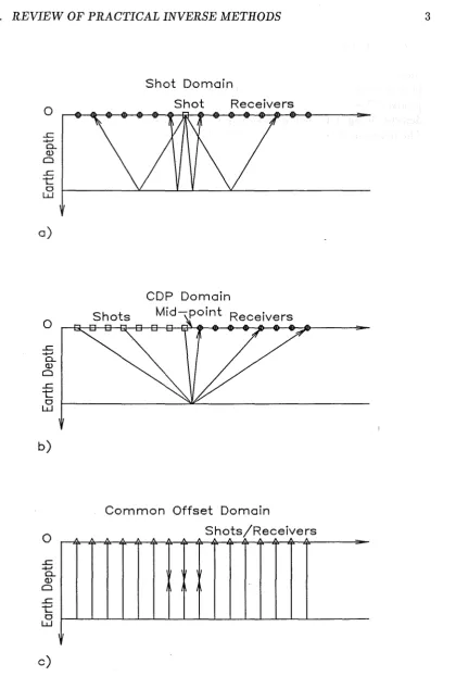
When a geological area is to be probed by seismic imaging, the shot holes and geophones must be appropriately located. They are commonly laid out as a linear array. The shot holes are usually equi-spaced along a particular line while the geophones are planted firmly on the ground on either side of the holes. Typical positions of the geophones with respect to a shot hole are shown in fig. 1.1a. After each shot the geophones are repositioned around the next shot in the same way. Recording equipment is connected to the geophones so that the data collected after each shot can be processed later.
o
...c:
-<-'
CL
Q)
o
...c:
'1:: o w
a)
o
...c:
-<-'
CL
Q)
o
...c:
'1:: o w
b)
o
...c:
...j..J
CL
Q)
o
...c:
'1:: o
w
c)
Shot Domain
Shot Receivers
CDP Domain
Common Offset Domain
[image:17.561.91.512.40.675.2]Shots/Receivers
4 CHAPTER 1. INTRODUCTION
to noise ratio for the resultant signals reflected from each point. The resultant signal represents a reconstruction of the reflectivity of the Earth along a vertical line below the centre of the observation structure. An image is built up of the Earth's reflectivity by reconstructing the reflectivity at adjacent vertical lines and mapping them appro-priately. The common depth point method is equivalent to the observation structure depicted in fig. 1.1c, but with an improved signal to noise ratio (Schoenberger, 1984). The .image so obtained can be used for geological exploration. However, a number of shortcomings of the cdp process have been recognised since it was originally introduced over 30 years ago. It is now common practice to carry out additional processing, after cdp stacking, to correct for some of the known shortcomings. The additional processing which is involved is discussed next.
The velocity of seismic waves near the surface of the Earth varies from point to point. Unless properly accounted for, these variations affect the quality of the recon-structed image (Schoenberger, 1984). Because the variations can usually -be inferred from geological bore hole studies (Schoenberger, 1984), their detrimental effect can be corrected. The variation in seismic velocity near the Earth's surface correspondingly alters the delay each reflected signal experiences before reaching a geophone. The vari-ations in delay cause the images of the reflecting points to be distorted. The distortions are corrected by time-shifting each recording by an amount governed by the known seis-mic surface velocity variations. These corrections are usually made when normal move out correction (introduced in the previous paragraph) is performed because both pro-cesses carry out time-shifting of the recorded signals. The resultant image represents an improvement because the reflecting points are more accurately positioned.
In the common point stack method it is assumed that the reflected signals received by each geophone are predominately from a single direction. Frequently, in fact, the seismic signal recorded by a single geophone is a superposition of seismic waves of comparable amplitude originating from a range of directions. A better description of the seismic data acquisition process is that of a recording of upward travelling waves emanating from points in the Earth. To produce an improved image using this descrip-tion the recordings in the cdp process are used to construct a field satisfying the wave equation (Sengbush, 1983). As a result, the recorded waves are propagated backward or migrated from the surface of the Earth to the reflector locations to produce a more faithful image. However the velocity of the seismic waves in the Earth must be known
a priori or assumed. This process has become known as migration and is usually
per-formed after normal moveout correction in cdp processing (Berg and Woolverton, 1986). Distortion of the image also occurs because the explosive shot does not produce an ideally sharp source pulse. The actual source pulse can be modelled as a convolution of an ideally sharp pulse with a known distorting function which is determined from the explosive type, shot position and the seismic recording itself (McQuillin et al., 1984).
Standard deconvolution techniques can be invoked for final enhancement of the image by reducing the effects of the distorting function (Sengbush, 1983).
1.1.2 Ultrasonic Methods in Medical Imaging
ment of foetal development during pregnancy (Wells, 1977). The growth in the use of ultrasound for medical diagnosis can be partly attributed to the current evidence that it is safe as compared to the known hazards of ionising radiation (Stratmeyer and Lizzi, 1986). However constant vigilance over its safety is warranted as our knowledge of thermal effects, cavitation and acoustic streaming and other biological phenomena increases. At high powers ultrasound has been shown to cause permanent changes to human tissue. These effects are harnessed, for example, in various surgical operations and physiotherapy (Wells, 1977). The most widely used ultrasonic imaging technique at present is B-scan which is able to provide a 2D image (Fatemi and Waag, 1983). This section describes the principles of the B-scan modality.
B-scan imaging relies on ultrasound being reflected from organs inside the body. The strengths and delays of the reflections enables the structures and positions of the body organs to be estimated (Halliwell, 1987).
The ultrasound for a B-scan medical instrument is normally generated by a piezo-electric transducer. The transducer is shaped so that it emits a narrow beam of ultra-sound. The ultrasonic frequencies are generally set in the 1 to 10 MHz range, which is chosen as a compromise between high resolution for the image and acceptable attenua-tion of the signal passing through body tissue (Taylor, 1979). The ultrasonic transducer also serves conveniently as a receiver because the piezo-electric effect is reciprocal.
The positioning of the transducer, on the surface of the body, for B-scan imaging is shown in fig. 1.2.1. A short pulse is transmitted from the transducer. The reflected signals caused by interaction of the ultrasound with the body are recorded by the same transducer. Because the transmitted pulse is emitted in a narrow beam, the observed signal characterises the reflectivity of the body along a small tube originating from the transducer (Wells, 1977).
The reflected signals are conveniently displayed on a cathode ray tube. The sig-nals are electronically mapped onto a line on the cathode ray tube which represents the reflectivity along the narrow beam of ultrasound emitted by the transducer (see fig. 1.2b). A complete 2D image of the body is built up by successively changing the direction ofthe transmitted beam and mapping the received signals onto corresponding lines on the cathode ray tube. Changing the direction of the transmitted beam can be effected mechanically but it is nowadays usually done electronically by using a phased array transducer (Taylor, 1979).
The interpretation of images produced by B-scan is difficult for untrained personnel. However, trained personnel are able to make accurate diagnoses from the images (Kim
et al., 1987).
1.1.3 Computed Tomography
6 CHAPTER 1. INTRODUCTION
r - - - - . . ,
Transducer
a)
Ib)
Figure 1.2: Operation of ultrasonic B-scan. a) The ultrasonic transducer is placed on the human body and the ultrasonic beam (dashed line) is electronically moved over a range of directions. b) An image of the reflectivity of the human body is displayed on a cathode ray tube. The solid dots correspond to points in the body which have caused the ultrasonic beam to be reflected.
tions to the field (Robb, 1985). During the 1980s, CT machines have been installed in a great many clinics and hospitals around the world (Herman, Ed.) (1983).
CT relies on tissues and tumours of different types attenuating x-rays differently. The attenuation an x-ray experiences while it passes through the body equals the in-tegral of the body's attenuation coefficient along the line the x-ray travels. In practice these integrals can be acquired by detecting the strength of x-rays, emitted by a source, which have transversed the human body. By collecting integrals through a cross-section of the body over a range of angles co-planar to the cross-section an image of the attenu-ation coefficient at each point in the cross-section can be obtained (Radon, 1917,Bates and McDonnell, 1989, Chapter 5). Because the attenuation of most materials is closely proportional to their materials densities the image of the cross-section's attenuation coefficients is effectively an image of the density (Bates and McDonnell, 1989, Chapter 5). Through this method CT is able to provide accurate quantitative reconstructions of densities of the cross-sections of bodies.
Commercial x-ray CT scanners generally comprise six modular subsystems (Robb, 1985). These are the gantry which supports the x-ray source and detectors, the moveable table on which the patient lies, the x-ray source, the array of detectors, the associated computer and the image display system.
/ I
I
\ \ I \ / ' /-
---"'-Source
"-\Body \
\ I
I
I /Detector
Array
Figure 1.3: Basic fan beam geometry used in modern CT scanners. A single x-ray source produces a fan beam of x-rays sensed by an array of detectors. Simultaneous rotation of the x-ray source and detector array through 3600 enable integrals of the attenuation coefficient through the body to be collected.
contribute to the reconstructed image. The design of the x-ray detectors is critical for the resolution and contrast, set by the sizes and efficiencies of detectors respectively, of images formed by CT scanners. Three types of detector which are commonly used are those termed scintillation, gas and solid state CRobb, 1985). Aperture diameters are between 0.75mm and 2.0 mm. The gantry provides rotational movement and supports the source and detectors. It is fabricated to strict mechanical tolerances to ensure precise alignment of the x-ray source and detectors relative to the body being imaged. Most modern CT gantries employ what is known as fan beam scanning, as illustrated in fig. 1.3. Simultaneous rotation of the x-ray source and detector array through 3600
enables a body's cross-section to be illuminated from all directions in the plane of the cross section. The data gathered for each direction of illumination corresponds to inte-grals of the body's cross-section attenuation along the paths of the x-rays. Fan beam scanning of a single cross section of a body can typically be completed in under five seconds.
Once the scan is completed the collected data must be processed to form an image. The data are treated as projections through the cross-section of the body so that algorithms based on the projection theorem can be invoked to generate an image of the cross-section (Bates and McDonnell, 1989). This involves converting around one million observations into a 256x256 or 512x512 pixel image. Today's minicomputers are able to perform this processing within a few seconds. Once the image has been computed it must be displayed. The display device is normally a cathode ray tube capable of 512 grey levels, or colour with 1024x1024 pixel resolution. Image manipulations, such as emphasising certain regions and producing histograms, are also possible and are now incorporated into commercially available display modules.
8 CHAPTER 1. INTRODUCTION
can be recognised by the untrained eye. It is this image quality which is characteristic of CT scanners (Robb, 1985).
1.2
Research Directions for Practical Inverse Methods
The desire to obtain more precise information about remote objects is seemingly insa-tiable. This section discusses some of the research directions being followed with the aim of improving the inverse methods which are presently invoked in practice.
1.2.1 Seismic Methods in Geophysics
One motivation for improving seismic imaging techniques is the increasing demand for oil world wide and the decreasing number of deposits available. More accurate techniques are required to discover whether oil deposits are likely to exist in terrain which is difficult to image and to form new images of regions which have been prospected with the aid of older techniques.
Historically, the first imaging techniques were based on assuming the earth could be modelled as a series of spherically symmetric layers. Earth structure departing radically from this model could not be imaged. Today, methods based on so-called migration techniques (see §1.1.1) can image asymmetrical or amorphous regions of the Earth, provided the local seismic velocities can be reasonably accurately obtained (Sen-gbush, 1983). If the estimated velocities are significantly erroneous, apparent positions of reflecting boundaries are seriously misplaced.
Another drawback of migration techniques is that the only property of the Earth which can be imaged is reflectivity. Specific rock types and densities can only be iden-tified after the images are interpreted in the light of geological expertise (Daily, 1986).
Direct recovery of acoustic or elastic parameters of the Earth, with little reliance on a priori information concerning the spatial variation of seismic velocity, is the
ulti-mate aim of all current research into seismic techniques (Lines, 1986). The approaches presently being investigated are perhaps better described as seismic inversion rather than seismic imaging. Such inversion techniques are based on full-wave descriptions of seismic propagation. However, they need considerable further development in order for them to be of routine practical use (Daily, 1986; Lines, 1986). The methods are very expensive computationally and more study is needed of their sensitivity to the cor-rupting effects of noise. Special geometries of the Earth structure must sometimes be assumed in order to generate apparently unique images. The majority of these methods are also predicated on seismic sources which give rise to plane waves, something which rarely occurs in practice. It is only when these shortcomings are overcome that it will be possible to claim that valid inversion techniques have been developed.
Because of the difficulties associated with seismic inversion research is also be-ing performed on inversion methods which incorporate adequate descriptions of wave motion (not necessarily full wave descriptions) and which are also manageable in prac-tice. Some of the research being pursued to this end has been reported by Lytle and Dines (1980), Clayton and Stolt (1981), Beylkin (1985), Devaney (1987) and Lo
et
Ultrasonic imaging has become the dominant imaging modality in many areas of med-ical diagnosis. However, comparison of ultrasound B-scan with x-ray CT images, for example, shows that the information displayed in B-scan images is much less quanti-tative. Although the initial development of ultrasonic B-scan was rapid, it has now reached a plateau without any significant recent technological advances having been reported (Moss, 1982).
Spatial resolution of B-scan is comparatively poor and the images contain speckle (Moss, 1982; Shankar, 1986). Quantitative interpretation of B-scan images, such as unambiguous characterisation of different types of tissue, is heavily dependent on the experience operators gain by experiment (Greenleaf, 1983). There is also a need for improved understanding of transducer operation so that specialised transducers can be designed for certain surgical operations (Moss, 1982).
Improvements in transducer design are allowing greater resolution by providing smaller beamwidths and narrower pulses. However, mere reliance on superior hard-ware must limit possible improvements in image quality (Fatemi and Waag, 1983; O'Donnell, 1988). This is because ultrasonic propagation can rarely be described, even approximately, in terms of straight rays (such as is permissible, in almost all instances, for radar). Phenomena such as diffraction and refraction cause the ultrasonic rays to deviate significantly from being straight. This suggests that imaging methods like B-scan, which are based on a straight ray model of ultrasonic propagation, can rarely be expected to produce faithful images. Substantial improvements in image quality will only be possible after a model of propagation which incorporates phenomena such as refraction and diffraction has been devised. When (and if) this is done, it should en-able images to be formed which quantitatively relate to some parameter characterising a physical property of the body (Greenleaf, 1983).
Ultrasonic imaging methods which are based on a full-wave description of propaga-tion have been developed by Roger (1981), Johnson and Tracy (1983), Colton (1984), Kristensson and Vogel (1986) and Colton and Monk (1988). They suffer, however, from certain drawbacks which prevent them being used in practice. Some of them demand large computational power whilst others can only accurately image a restricted set of objects. As in seismic imaging, there is a need for techniques which can combine an adequate description of wave motion with practical exigencies. Relevant studies are pre-sented by Bates et al. (1976), Beylkin (1985a), Dines and Goss (1987), Devaney (1987),
Schultz and Jaggard (1987).
1.2.3 Computed Tomography
CT has become the standard to which a number of other imaging techniques are com-pared. However, there are certain aspects of CT images which medical practitioners would like to see improved.
10 CHAPTER 1. INTRODUCTION
The problems mentioned above are mainly due to comparatively large detector beamwidths, non-monochromatic x-ray sources and relatively slow scanning times, which can, in principle, be remedied by improved hardware. The fundamental model upon which CT is based closely approximates the basic physics. This means that im-provements in the imaging hardware, rather than the propagation model, are more likely to result in improvements in image quality. This contrasts markedly with many otherinverse methods which require improvements to their models of wave propagation.
1.3 Archetypal Problems
Having descriptively examined, in §1.1, some inverse problems which occur in practice, it is now appropriate to formally define a general, or archetypal, inverse problem (see §1.3.3). Inverse problems can only be systematically analysed if they are presented within a general mathematical framework. Mathematical analysis of such problems allows reliable solutions to be obtained, where the term reliable here implies that the levels of validity of the solutions, and the conditions under which they can be invoked, can be quantitatively characterised. Since inverse problems can only be understood in the contexts of their associated direct problems (recall that both inverse and direct problems have been discussed in general terms in the preface) an archetypal direct prob-lem is also formulated in this section (see §1.3.2). Terminology and notation suitable for such a framework are introduced in §1.3.1.
1.3.1 Terminology and Notation
It is convenient to partition K-dimensional space as indicated in fig. 1.4. Although this thesis is only concerned in detail with K=3 and K=2, it seems appropriate to start out in this section by establishing notation for a space of arbitrary dimensionality. The whole of K-dimensional space is denoted by 1, an arbitrary point in which is labelled by the position vector x with respect to an arbitrarily chosen coordinate origin 0. The scattering region (taken to be finite) is denoted by 1_, the surface of which denoted by 0". The hyper-spherical surface 0"_ centred on 0, inscribing 1_, partitions I_into 1 __ and 1_+ interior and exterior, respectively, to 0"_. The part of 1 exterior to 0" is denoted by 1+. The hyper-spherical surface 0"+ centred on 0, circumscribing 1_, partitions 1+ into 1+_ and 1++ interior and exterior, respectively, to 0"+. Invoking set theoretical notation, the above definitions are formalised by
1 = 1_ U 0" U 1+ and 1 _
n
0" = 1+n
0" =0
(1.1) where0
is the empty set, with(1.2)
and
1+ = 1+_ U 0"+ U 1++ and 1+_
n
0"+ = 1++n
0"+ =0
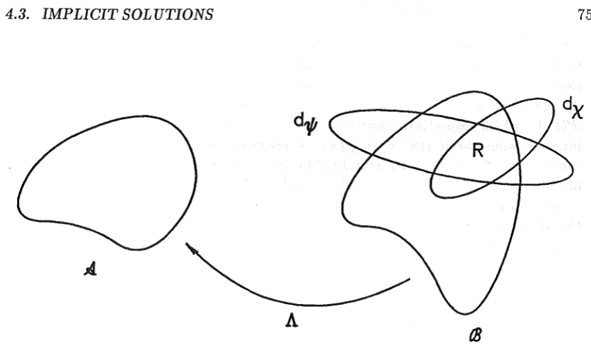
(1.3) The generalised constitutive parameter X characterises properties of interest within--n-;'
"-/
"-/
"
/
"-I - ff_- - '\
/ "- \
/ \
I
1 __
\I
\0
\ lobs•
I
I
\
I
\ \ I
\ /
\ / I
"
----
I'\
1+_
"-
/"
"- / /"- ...
.,,-
----'f.:
+- - -
--1++
Figure 1.4: Partitioning of space. The symbols T and (J' refer to hyper-volumes and
12 CHAPTER 1. INTRODUCTION 1/Js. The latter emanation results from the probing emanation interacting with the generalised constitutive parameter. Therefore
(1.4) The regions Tine and T obs are where, respectively, the sources of the incident ema-nations reside and the scattered emaema-nations are observed. Both of these regions are defined to be outside T _, so that
Tine C T++ and Tobs C T++ (1.5) It is emphasised that both two-dimensional (K=2) and three-dimensional (K=3) scattering can be conveniently described with the aid of the above notation. In general, when K=3, T _ is a conventional volume of arbitrary shape, with 0'_ and 0'+ being
conventional spherical surfaces. Now consider the special situation of T-_ being an infinite cylinder of arbitrary cross-section (whose shape is defined by 0' which in this
instance is of course a cylindrical surface). If, in addition, 1/Ji exhibits no variations in the direction of the cylinder's axis (e.g. it is a plane or cylindrical wave oriented appropriately to this axis) then 1/J only varies in directions lying in planes perpendicular to the said axis, implying that the scattering is effectively two-dimensional.
When the scattering is effectively two-dimensional, as indicated in the previous paragraph, it can be treated mathematically as actually two-dimensional (i.e K=2). Then 0' reduces to an arbitrary closed curve, with 0'_ and 0'+ being perimeters of circles
centred on the origin 0 of coordinates. In later Chapters it is often found convenient (when K can be taken to be 2) to accord to x the Cartesian coordinates
(x, y)
and the cylindrical polar coordinates (Pi<fJ),
or alternatively (ri 0).1.3.2 The Direct Problem
The direct problem is here stated as
(1.6)
where A is an operator which describes the interaction of the emanations with the generalised constitutive parameter X. The direct problem can consequently be alter-natively stated as: given the generalised constitutive parameter, calculate the result of interactions of the emanations with it.
This definition and the terminology introduced in §1.3.1 are adequate for specifying most direct problems of practical interest. For example, the associated direct problem for ultrasonic B-scan is to calculate 1/Js in T obs which is the exterior surface of the ul-trasonic transducer. The scattering region T _ is the body, the generalised constitutive parameter is the body's reflectivity, and the emanations are ultrasonic waves. The probing emanations originate from the ultrasonic transducer, the exterior surface of which is also Tine.
1.3.3 The Inverse Problem
The inverse problem is the mathematical inverse of (1.6) and is stated here as
domain of X is within T _, whereas 'IjJ can only be observed in practice within Tobs.
The inverse problem can consequently alternatively be stated as: given the emana-tions within T obs, calculate the distribution of the generalised constitutive parameter
throughout T_.
This definition and the terminology introduced in §1.3.1 are adequate for specifying many inverse problems of practical interest. For example, when inverting seismic data (Le. forming seismic images) the scattering region T _ is the Earth, the generalised constitutive parameter is reflectivity, and the emanations are seismic waves. The region
Tine is where the apparatus which generates the shots is. As explained in §1.1.1, these shots are the source of the probing emanations. The scattered emanations are the reflected signals which are observed at the geophones in the region T obs. Seismic
imaging thus involves determining the reflectivity of the Earth from seismic observations made outside the Earth.
All this can be summarised. The direct problem can be considered as, given a cause find the effect, whilst the inverse problem is, given an effect find the cause.
1.4
Solving the Inverse Problem
The inverse problem is mathematically defined in (1.7). The solution to (1.7) in specific situations represents mathematical descriptions of imaging methods. To find a solution to (1.7), the operator A -1 must first be specified. The form of A -1 depends on the
underlying physics of the interaction of the emanations with the generalised constitutive parameter X. In most situations, X can only be expressed as an implicit non-linear function of 'IjJ, mainly because 'ljJs can only be observed outside the body whereas X
exists entirely inside the body. Solutions deduced from A -1 can usually be expected
to be either non-unique, non-existent, or to depend non-continuously on the data. An operator characterised by one or more of these properties is ill-posed (Baltes, 1980; Sabatier, 1983). An ill-conditioned system is here defined to be a system that manifests itself numerically as the consequence of either an ill-posed operator or an operator which is nearly so.
Ill-posedness can usually be ameliorated by regularisation which can be regarded as a technique for incorporating a priori information to restrict the set of possible solutions (Baltes, 1980; Sabatier, 1983). There are two commonly adopted approaches which overcome the inherent implicit and non-linear nature of A -1. One either introduces
approximations to reduce A -1 to a explicit linear expression or one invokes inversion
theory (Sabatier, 1983). These two approaches are discussed next.
Approximations can be invoked which enable the operator A -1 to be expressed
such that it depends explicitly and linearily on the scattered field. A solution to the inverse problem is then obtained by directly evaluating the operator. The structure of the corresponding direct problem is usually invoked to develop an explicit linear expression for A -1. This is effected by approximating the direct problem to obtain an
14 CHAPTER 1. INTRODUCTION
approximation has yet been found) without generating wildly inaccurate solutions. For example, seismic and ultrasonic imaging techniques sometimes produce severely distorted images because the operators involved are being approximated poorly. In the case of CT, however, only small approximations to the operator are required with the result that the images produced are relatively undistorted.
The other approach which overcomes the implicit non-linear nature of A-I is to invoke what is called inversion theory (Rall, 1969; Sabatier, 1983). This approach is based on the notion that A which is the operator for the direct problem, maps the generalised parameter X to the scattered field 1/;8' This suggests that a model of the unknown X can be guessed, so that the corresponding field 1/;8 can be calculated. If the calculated scattered field is sufficiently close to the observed 1/;8 then X can be said to be a solution to the inverse problem. If 1/;8 is not sufficiently close to the observed scattered field then X must be altered until 1/;8 becomes sufficiently close. This idea leads to a general iterative solution to inverse problems which hopefully locates correct solutions. A thorough understanding, however, of the underlying physics is necessary to ensure satisfactory solutions are obtained (Baltes, 1980; Sabatier, 1983)
Because, in both of these approaches, the direct problem plays a central part in the solution of the inverse problem, it is important to understand the analytical niceties of the direct problem. Accordingly, Chapter 3 is devoted to the direct problem.
1.5
Impact of Dimensionality of Space on Inverse
Prob-lems
There is a considerable literature on inverse scattering problems posed in one spa-tial. dimension. Some key references are Gelfand and Levi at an (1955), Chadan and Sabatier (1977) Newton (1981) Hashaby and Mittra (1987) and Bruckstein and Kailath (1987).
Study of the references quoted above reveals that one-dimensional inverse scattering theory is by now comparatively complete and very well understood, which contrasts spectacularly with the state of the general theory for more than one spatial dimension. There are two reasons for this (Bates
et ai.,
1990).There is a physical intuition concerning the interaction of linear wave motion with scatterers, which is so ingrained in radio/radar engineers, acousticians and quantum physicists, that it must essentially characterise natural wave phenomena in the great majority of physically interesting situations. This intuition claims that wave scattering can be represented in terms of rays. That is, wave motion penetrates a body in such a way that the energy propagates along curves. In one dimension then, one knows a
priori the directions of all rays for a one-dimensional inverse scattering problem. There
is only one direction (Le. that corresponding.to the single spatial dimension) in which they can travel! In more than one dimension the rays travel along arbitrary curves which are not known a priori. Consequently, the inverse problem acquires an extra
degree of intricacy in more than one dimension.
It can be immediately appreciated from the above that the technical (due to not being able to transform to the equivalent of the Schrodinger equation) and concep-tual (associated with being unclear a priori as to the actual ray paths) difficulties
Mathematical Preliminaries
This Chapter is concerned with the various mathematical techniques, together with their associated terminology and notation, which are needed for solving direct and inverse problems involving wave-like emanations. Actual solutions to these types of problem are presented in Chapters 3,4 and 5. These mathematical preliminaries provide the proper setting for the later Chapters and allow the solutions to be developed without unduly disrupting them to make every point precise.
An important preliminary is to find the form of the operator A describing the inter-actions between the wave-like emanations and the generalised constitutive parameter (see §1.4). In §2.1 mathematical models are developed for describing these interactions through differential equations. The applicability of the models is discussed and their formulation in the time and frequency domains are presented. The relative merits of the time and frequency domain formulations are also discussed. §2.2 presents vari-ous supplementary definitions and mathematical techniques which are useful in solving direct and inverse problems.
2.1
Mathematical Models of the Physics of Scattering
Wave motion in various media can be modelled by differential equations. The wave motion can be formulated in either the time domain or the frequency domain.
2.1.1 Time Domain Formulations
Under certain sets of conditions, applying in many situations of practical interest, electromagnetic, elastic and acoustic emanations can be described by a common math-ematical model. These emanations can be adequately represented in the time domain by a complex valued scalar wave function
W(x,
t), hereafter called the field, which ex-ists at all points x E T in arbitrary dimensional space and all instants t ERin time (Felson and Marcuvitz, 1973, Chapter 1). Any individual Cartesian component of a vector field can also be described byW(x,
t)
provided there is negligible cross coupling between the field's components. The Cartesian coordinate in the direction of the chosen component of the vector field is denoted bye. When the medium is source free, linear, time invariant and isotropic, the emanations can be described by the partial differential equation .V2W(X,
t) - ,6(x)W(x, t) -
(v(x)jc?W(x,t)
+
p(x)W(x,
t)
=0
(2.1)18 CHAPTER 2. MATHEMATICAL PRELIMINARIES
where c is the free-space wave speed and
(3(x), J.L(x)
andvex)
are constitutive parameters which are related in table 2.1 to the properties ofthe medium for each type of emanation (Morse and Feshbach, 1953, Chapter 2; Born and Wolf, 1970, Chapter 1). Table 2.2 lists the symbols used in this thesis to represent properties of the media.Emanation
I
(3(x)
I
J.L(x)
I
vex)
I
Electromagnetic
J.LoU
0I~:
Elastic 0 2e.V2e.-3Ve..Ve. 4p2
Jf
Acoustic 0 2e.V2e.-3Ve..Ve. 4p2J~
Table 2.1: Constitutive parameters
(3(x), J.L(x)
andvex)
related to the properties (them-selves listed in Table 2.2) of propagating media for electromagnetic, elastic and acoustic wave motion.Property
I
SymbolI
Free-space permeability
J.Lo
Permittivity f.
Free-space permittivity f.o
Electrical conductivity u
Density p
Compression modulus K
Bulk modulus A
Table 2.2: Properties of media and the respective symbols used to represent them.
To derive the relationships between the properties of the medium and the consti-tutive parameters, certain limitations on the medium must be imposed for each type of emanation. These limitations imply that (2.1) is only valid under restricted sets of conditions. These conditions are, however, of considerable practical interest.
To allow electromagnetic emanations to be described by (2.1),
W(x,
t)
is taken to represent a single component of the electric or magnetic field. Because the great ma-jority of media are non-magnetic, negligible error results in general from assuming the permeability of the medium to be constant and equal to its free-space valueJ.Lo.
A more significant limitation is that the permittivity f. cannot be allowed to exhibit appreciable spatial variations in the ~-direction. The implication here is thatV'(W(x,
t)
ge
loge f. must be everywhere small compared with bothV'2W(X,
t)
and c~W(x,
t)
(Jones, 1964, Chapter 1; Born and Wolf, 1970, Chapter 1). While the class of media that satisfies this limitation is palpably restricted, it is wide enough to be of considerable practical interest.belong to the class for which there is negligible shear in the ~-direction (Spencer, 1980). It is thus seen that the limitations on the allowable classes of media are similar for electromagnetic waves and elastic shear waves.
Acoustic emanations can also be described by (2.1) if
W(x,
t)
represents the velocity potential for the particles in the medium (Wilcox, 1984, Chapter 1). Since acoustic emanations can also occur in p and s forms, the viscosity of the medium must be effectively zero so that there is negligible transformation of energy between acoustic pressure waves and shear waves.2.1.2 Frequency Domain Formulations
Because (2.1) is linear in
W(x,
t),
an equivalent description of the emanations can be formulated in the temporal frequency domain §2.2.6. The emanations can then be described by'Ij;(x,
k) which is the temporal Fourier transform ofW(x,
t), The differential equation for'Ij;(x,
k) is obtained by Fourier transforming (2.1), thereby producing the Helmholtz wave equation (Morse and Feshbach, 1953, Chapter 11) equation(2.2)
Although the wave equations (2.1) and (2.2) are exactly equivalent, the latter is in a important sense more versatile because the three constitutive parameters appearing in (2.1) can be combined in the frequency domain into a single generalised constitutive pa-rameter, written here as X
=
X(x, k). Then, (2.2) can be simplified, and simultaneously generalised, to(2.3)
where
The first term on the right hand side of (2.4), which is independent of k, determines the speed of the wave motion at each point in the medium. The square root of this term is what is known historically as the refractive index.
In free space
J.L(x)
=
(3(x)=
0 andvex)
=
1. The wave equation then becomes(2.5)
which is known as the free-space wave equation.
2.1.3 Comparison of Time and Frequency Domain Formulations This section compares time domain and frequency domain formulations thereby allow-ing the advantages and disadvantages of each formulation to be highlighted.
20 CHAPTER 2. MATHEMATICAL PRELIMINARIES
unstable numerically. On the other hand, frequency domain formulations can allow several different characteristics of a medium to be combined into a single constitutive parameter, as is manifested by (2.4). For example, dispersion and attenuation, charac-terised by ",,(x) and f3(x) respectively, which have to be inserted separately into time domain formulations, can be combined in the frequency domain by permitting X(x, k) to be complex and frequency dependent.
From a theoretical point of view, time domain and frequency domain formulations are equivalent. However, the numerical difficulties arising from time domain approaches can be daunting. Consequently, as is in accordance with the majority of the current literature on inverse problems, this thesis concentrates exclusively on frequency domain formulations.
2.2
Supplementary Definitions and Mathematical
Tech-.
nlques
This section is a collection of concepts, definitions and mathematical techniques which are made use of later in the thesis. As is conventional, "right hand side" and "left hand side" are abbreviated to RHS and LHS respectively, and Re and 1m are the abbreviations for "real part" and "imaginary part" respectively.
2.2.1 Partitioning of Wave Motion
The incident and scattered fields are partitioned according to (1.4). The most .conve-nient definition of the incident field is to make it a solution of (2.5) in all of space apart from Tinc, where the sources of the incident field reside. This then forces "pi(X, k) to be a solution of
(2.6)
everywhere except within Tinc, so that (2.3) becomes
(2.7)
Because LHS (2.7) has the same form as that of the free-space wave equation (2.5), the negative of the RHS can be considered to be a density of equivalent sources embedded in free-space. The field emanating from these sources constitutes the scattered field.
A particularly convenient type of incident radiation is the plane wave. It can be written as
(2.8)
where the direction of propagation is specified by the unit vector
k
= k/k. Surfaces of constant complex amplitude are specified as .in two dimensions in this thesis. Specific two-dimensional forms of the plane wave are consequently needed. If the arbitrary point x is accorded the cylindrical coordinates
(Pi </» then (2.8) can be expressed a
1/J(Pi </>, k) = e-jkp cos(t/>-O) (2.10)
where () specifies the direction of propagation of the plane wave.
A multipole expansion can also be invoked to represent the planar incident field. When this is done, (2.8) becomes (Jones, 1964, Chapter 8)
00
1/Ji(x,k)
=
1/Ji(p;</>,k) =I:
amJm(kp)eimt/>(2.11)
m=-oo
where Jmc-) is the Bessel function of the first kind of order m, and the am depend on the direction of propagation through am = (_j)me-jmO.
2.2.2 Far-field (Fraunhofer region) Conditions
In perhaps the great majority of practical applications of inverse scattering, T aba lies
in what is called the far-field, or Fraunhofer region, of T _. Consider an arbitrary point
PET aba and any two points pi and P" lying in T _. The essence of the far-field
approximation is that the straight lines pip and P" P can be taken with negligible error to be parallel. This means that the actual value of ~
=
IP' P - P"PI
is negligibly different from what it would be if P was infinitely distant from T _. What actuallymatters, of course, is how large ~/,\ is, where ,\ is the free-space wavelength of the wave motion. If L is the maximum transverse dimension of T _, as seen from P, then
~ ~ L2/8R, where R
=
P pi averaged over all pi E T _. Radio-engineering folk-lore(Le. what antenna engineers have found by experience, over the past 50 or so years, to be appropriate) is that ~ should not exceed '\/16, which implies the far-field distance
is 2L2 /,\ (Goodman, 1975, Chapter 1; Blake, 1984, Chapter 6) If ,\/16 is considered
too large a value for ~ in a certain application then the distance must be increased, but not necessarily by much since ~ varies as 1/ R2.
2.2.3 Characterisation of Scattering
The relative strength of the scattered field compared to the incident field is an important factor in many situations. It is convenient to classify the "strength" of the scattering as very weak, weak or strong. To formalise the classification it is necessary to define the quantities
Adijj(X, k) = I¢(x, k)I-I¢i(X, k)1
(2.12)
which is here called the amplitude increment, and
Phdiff(X, k)
=
L¢(x, k) - L¢i(X, k)(2.13)
which is called the phase increment, where Lq denotes the phase of q. The incremental phase change ~(x, Xl, k) between points X and
X:I
is defined to be22 CHAPTER 2. MATHEMATICAL PRELIMINARIES
Very weak scattering can then be said to occur when AdiJ J ~ 0 throughout i_and
~(X,XI' k)
<
I
for all pairs of points x and Xl at which rays of'l/Ji
enter and leave i _. Recall that the concept of rays is introduced descriptively in §1.5. It is made more precise in §2.2.1.Weak scattering is defined similarly to very weak scattering except that x and Xl are points on rays of
'l/Ji
separated by A.Strong scattering occurs when, within an appreciable fraction of i _, AdiJJ differs significantly from zero and/ or ~(x, XI, k) is appreciably greater than
I
for points X and Xl on rays of'l/Ji
separated by A.2.2.4 The Green's Function
The Green's function is defined as the particular solution of the equation
(2.15)
where the quantity g(x, Xl, kv) is called the Green's function for the operator (\72
+
k2v2 ) (Morse and Feshbach, 1953, Chapter 6). Physically, it represents the field at the
point X radiated from a point source of unit strength at Xl. Writing Ix - XII = T, it
transpires that the two- and three-dimensional forms of g(x, Xl, kv) are (Jones, 1964, Chapter 1)
(2.16)
where
Hg2)(.)
is the cylindrical Hankel function of the second kind of order zero, and R K denotes the set of points in K -dimensional space.For the reasons given in §1.5, it can be appropriate as well as convenient to illustrate numerical aspects of inverse methods in two dimensions. If the a!bitrary points X and Xl are accorded the cylindrical polar coordinates (Pi </» and (Ti 8) in two d