Solving Short Term Multi Chain Hydrothermal Scheduling Problem by Artificial Bee Colony Algorithm

© 2015 IJSRST | Volume 1 | Issue 3 | Print ISSN: 2395-6011 | Online ISSN: 2395-602X Themed Section: Engineering and Technology

Solving Short Term Multi Chain Hydrothermal Scheduling

Problem by Artificial Bee Colony Algorithm

S. M. Abdelmaksoud, Ayman Y. Yousef, H. A. Henry

Department of Electrical Engineering Faculty of Engineering at Shoubra, Benha University, Cairo, Egypt

ABSTRACT

This paper presents an artificial bee colony algorithm for solving optimal short term hydrothermal scheduling problem. To demonstrate the effectiveness of the proposed algorithm, hydrothermal test system consists of three thermal units and four cascaded hydro power plants has been tested. The valve point loading effect is taken into consideration. In order to show the feasibility and robustness of the proposed algorithm, a wide range of thermal and hydraulic constraints are taken into consideration. The numerical results obtained by ABC algorithm are compared with those obtained from other methods such as genetic algorithm (GA), simulated annealing (SA), evolutionary programming (EP) and constriction factor based particle swarm optimization (CFPSO) technique to reveal the validity and verify the feasibility of the proposed method. The experimental results indicate that the proposed algorithm can obtain better schedule results with minimum execution time when compared to other methods. Keywords: Hydrothermal Generation Scheduling, Artificial Bee Colony, Valve Point Loading Effect

I.

INTRODUCTION

The hydrothermal scheduling problem is a non linear programming problem including a non linear objective function and subjected to a mixture of linear and non linear operational constraints. Since the operating cost of hydro electric power plant is very low compared to the operating cost of thermal power plant, the integrated operation of the hydro and thermal plants in the same grid has become the more economical [1]. The primary objective of the short term hydrothermal scheduling problem is to determine the optimal generation schedule of the thermal and hydro units to minimize the total operation cost of the system over the scheduling time horizon subjected to a variety of thermal and hydraulic constraints. The hydrothermal generation scheduling is mainly concerned with both hydro unit scheduling and thermal unit dispatching. Since there is no fuel cost associated with the hydro power generation, the problem of minimizing the total production cost of hydrothermal scheduling problem is achieved by minimizing the fuel cost of thermal power plants under the various constraints of the system [2]. Several mathematical optimization techniques have been used to solve short

system. The ABC algorithm is a population based optimization technique proposed by Devis Karaboga in 2005. It mimics the intelligent behaviour of honey bees. In ABC algorithm, the colony of artificial bee consists of three groups of bees: employed bees associated with specific food sources, onlooker bees watching the dance of employed bees within the hive to choose a food source and scout bees searching for food sources randomly. Both scouts and onlookers are also called unemployed bees. The first half of the colony consists of the employed artificial bees and the second half includes the onlookers. Compared to other evolutionary computation techniques, the ABC algorithm is simple and robust and can solve optimization problems quickly with high quality solution and stable convergence characteristic.

II.

Objective Function and Operational

Constraints

The main objective of short term hydro thermal scheduling problem is to minimize the total fuel cost of thermal power plants over the optimization period while satisfying all thermal and hydraulic constraints. The objective function to be minimized can be represented as follows:

T N

t t

T t _{i gi}

t=1 i=1

F =



n F (P )

(1) In general, the fuel cost function of thermal generating unit i at time interval t can be expressed as a quadratic function of real power generation as follows:

t t _i( t 2 _i t _i

i gi gi gi

F (P )=a P ) +b P +c

(2)

Where Pgit _{is the real output power of thermal generating}

unit i at time interval t in (MW), F (P ) t t

i gi _{is the} operating fuel cost of thermal unit i in ($/hr), FT is the total fuel cost of the system in ($), T is the total number of time intervals for the scheduling horizon, nt is the numbers of hours in scheduling time interval t, N is the total number of thermal generating units, a ,bi i_{and ci are}

the fuel cost coefficients of thermal generating unit i. By taking the valve point effects of thermal units into consideration, the fuel cost function of thermal power plant can be modified as:

t t _i( t 2 _i t _{i i i} min t

i,v gi gi gi gi gi

F (P )=a P ) +b P +c + e ×sin(f ×(P -P )) (3)

Where

t t i,v gi

F (P )

is the fuel cost function of thermal unit i including the valve point loading effect and fi, ei are the fuel cost coefficients of generating unit i with valve point loading effect.

The minimization of the objective function of short term hydrothermal scheduling problem is subject to a number of thermal and hydraulic constraints. These constraints

include the following:

1) Real Power Balance Constraint: The total active power generation from the hydro and thermal plants must be equal to the total load demand plus transmission line losses at each time interval over the scheduling period.

N M

t t t t

D L

gi hj

i=1 j=1

P  P =P + P





(4)

Where,

t D P

is the total load demand during the time

interval t in (MW),

t hj

P

is the power generation of hydro

unit j at time interval t in (MW),

t gi

P _{is the power}

generation of thermal generating unit i at time interval t

in (MW), M is the number of hydro units and

t L P represents the total transmission line losses during the time interval t in (MW). For simplicity, the transmission

power loss is neglected in this paper.

2) Thermal Generator Limit Constraint: The inequality constraint for each thermal generator can be expressed as:

min t max

gi gi gi

P P P

(5)

Where

min gi

P

and

max gi

P

are the minimum and maximum power outputs of thermal generating unit i in (MW), respectively.

3) Hydro Generator Limit Constraint: The inequality constraint for each hydro unit can be defined as:

min t max

hj hj hj

P P P

(6)

Where

min hj

P

and

max hj

P

4) Reservoir Storage Volume Constraint:

min t max

hj hj hj

V V V

(7)

Where

min hj

V

and

max hj

V

are the minimum and maximum storage volume of reservoir j, respectively.

5) Water Discharge Rate Limit Constraint:

min t max

hj hj hj

q q q

(8)

Where

min hj

q

and

max hj

q

are the minimum and maximum water discharge rate of reservoir j, respectively

6) Initial and Final Reservoir Storage Volume Constraint: This constraint implies that the desired volume of water to be discharged by each reservoir over the scheduling period should be in limit.

begin

0 max

= =

hj hj hj

V V V

(9)

T end

=

hj hj

V V

(10)

Where

begin hj

V

and

end hj

V

are the initial and final storage volumes of reservoir j, respectively.

7) Water Dynamic Balance Constraint: The water continuity equation can be represented as:

uj

uj uj R

t t-1 t t t t- _,

t-u u

hj hj hj hj hj u=1

V = V + I - q - S +



(q  + S  )

(11)

Where

t hj

I

is water inflow rate of reservoir j at time

interval t,

t hj

S

is the spillage from reservoir j at time interval t, τuj is the water transport delay from reservoir u to reservoir j and Ruj is the number of upstream hydro reservoirs directly above the reservoir j.

8) Hydro Plant Power Generation Characteristic: The hydro power generation can be represented by the following equation:

1j 2j 3j 4j 5j 6j

t ₍ t 2 ₍ t 2 ₍ t t ₍ t ₍ t

hj hj hj hj hj hj hj

P =C V ) +C q ) +C V )(q )+C V )+C q )+C (12)

Where C1j, C2j, C3j, C4j, C5j and C6j are the Power generation coefficients of hydro generating unit j

III.

Overview of ABC Algorithm

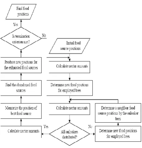
Artificial bee colony (ABC) is one of the most popular swarm intelligence algorithms for solving constrained and unconstrained optimization problems. It was first developed by Karaboga in 2005, inspired intelligent behaviors of real honey bee colonies [25]. The algorithm simulates the intelligent foraging behaviour of honey bees to achieve global optimum solutions for different optimization problems. The foraging behaviour of bees is to collect nectar from food sources around the hive in nature. In ABC algorithm, the position of food sources represents a possible candidate solution to the optimization problem, and the nectar amount of a food source corresponding to the profitability of associated solution. In ABC algorithm, the number of employed bees is equal to the number of food sources existing around the hive. If an employed bee could not improve the self solution in a certain time, it becomes a scout bee and the main purpose of which is to increase search ability of the ABC algorithm. The scout bees carry out a random search process for discovering new food sources. Compared to the other swarm based algorithms, the ABC algorithm has become very popular and it is widely used, because of its good convergence properties.

IV.

Search Mechanism of ABC Algorithm

The colony of artificial bees consists of two groups of bees called employed bees and unemployed bees. The unemployed bees consist of onlookers and scouts. The main steps of the ABC algorithm are explained as follow:

1) Initialize a randomly food source positions by the following equation:

X =X

ij jmin

+r×(X

jmax

- X

jmin

)

(13)

Xi={xi1, xi2, …….,xiD}, i = 1,2,….., Ns , j = 1,2,...,D

Where Ns is the number of food sources; D is the number of decision variables. R is uniformly distributed random value between [0, 1], Xj

min

and Xj max

2) Each employed bee searches the neighborhood of its current food source to determine a new food source using Equation (14):

V =X + ×(X - X )ij ij



ij ij kj (14)

Where:

k {1,2...,Ns} , j {1,2...,D} are randomly chosen indexes. It must be noted that k has to be different from i.



ij is a uniformly distributed real random number

between [-1, 1], it controls the production of neighbor food sources around Xij and represents the comparison of

two food positions visually by the bee.

If the new food source position produced by Equation (14) which exceeds their boundary values, it can be set as follow:

If X Xi > imax then

X X

i = imax

If X Xi < imin then

X X

i = imin

3) After generating the new food source, the nectar amount of food sources will be evaluated and a greedy selection will be performed. If the quality of the new food source is better than the current position, the employed bee leaves its current position and moves to the new food source, otherwise, the bee keeps the current position in the memory.

4) The onlooker bee chooses a food source by the nectar information shared by the employed bee, the probability of selecting the food source i is calculated by the following equation:

NS

j=1

fiti i=

fitj

P



(15)

After selecting a food source, the onlooker generates a new food source by using equation (14). Once the new food source is generated it will be evaluated and a greedy selection will be applied same as the case of employed bees.

5) If the solution represented by a food source position cannot be enhanced for a predetermined number of trials (called limit), the food source is abandoned and the employed bee associated with that food source becomes a scout. The scout generates a new food source randomly using the following equation:

min max min

ij j j j

V =X +r×(X - X )

Where j {1,2...,D} (16) 6) If the termination criterion is satisfied (maximum number of cycles), the process is stopped and the best food source is reported; otherwise the algorithm returns to step 2.

The schematic diagram shows the mechanism search of ABC algorithm is illustrated in “Fig. 1”.

Figure 1: Schematic outline of ABC algorithm

V.

ABC Optimization for Short term

Hydrothermal Scheduling Problem

The artificial bee colony algorithm for solving short term hydrothermal scheduling problem is described as follow:

A. Construction of Solutions

In the initialization process, a set of food source positions are created at random. In this paper, the construction of solution for short term hydro thermal scheduling problem is composed of a set of elements which represent the water discharge rate of each reservoir and the power generation of thermal units over the whole scheduling period. Thus, the structure of solution is defined as follows:

0 0 0 0 0 0

h1 h2 hj g1 g2 gi

1 1 1 1 1 1

h1 h2 hj g1 g2 gi

T T T T T T

h1 h2 hj g1 g2 gi

q q ...q P P ...P

q q ...q P P ...P X =

q q ....q P P ...P

 

 

 

 

 

 

 

M M O M M M O M

In the initialization process, the ABC algorithm generated the initial solutions by using the Equations (18) and (19) defined below.

t min max min g

gi gi gi gi

P =P

+r ×(P

-P

)

(18)

q =q

t_hj min_hj

+r ×(q

h max_hj

-q

min_hj

)

(19)

Where rg and rh are uniformly distributed random real

numbers in the range [0, 1]; i = 1,2,……,N , j = 1,2,…….,M and t = 1,2,……,T

The feasible candidate solution of each element must be initialized within the feasible range.

The elements t gi

P and t hj

P are the output power generation of thermal unit i during the time interval t and the water discharge rate of hydro unit j at time interval t, respectively. The range of the elements t

gi

P and t hj

P

should satisfy the generating capacity limits of thermal generators and the water discharge rate constraints.

If any food source position is not satisfy the constraints, then the position of the food source is fixed to its minimum and maximum operating limits as follows:

t min t max

gi gi gi gi

t min t min

gi gi gi gi

max t max

gi gi gi

P if P P P

P P if P P

P if P P

  



_   _ 

--- (20)

t min t max

hj hj hj hj

t min t min

hj hj hj hj

max t max

hj hj hj

q if q q q

q q if q q

q if q q

  



_   _ 

--- (21)

t min t max

hj hj hj hj

t min t min

hj hj hj hj

max t max

hj hj hj

V if V V V

V V if V V

V if V V

  



_   _ 

--- (22)

B. Evaluation of Fitness of Solutions:

Evaluate the fitness value of each food source position corresponding to the employed bees in the colony using the objective function described in Equation (1).

C. Modification of Food source positions by Employed Bees:

Each employed bee produces a new food source position by using equation (14). The modified position is then checked for constraints defined in Equations (5) and (8). If the new solutions violate the constraints, they are set

according to Equations (20) and (21). Then compute the fitness value of the new food source positions using Equation (1). The fitness of the modified position is compared with the fitness of the old position. If the new fitness is better than the old fitness, the employed bee memorized the new position and forgets the old one; otherwise, the employed bee keeps the old solution.

D. Sending the Onlooker Bees for Selected Positions and Evaluate Fitness:

Place the onlooker bees on the food sources with the nectar information shared by employed bees. Each onlooker bee chooses a food source based on the probability described in Equation (15). Onlooker bees search the new food sources in the neighborhood with the same method as employed bees.

E. Modification of Food Source Positions by Onlooker Bees:

The onlooker bees produce a modification on the position in its memory using Equation (14). Check the inequality constraints of the new positions. If the resulting value violates the constraint, they are set to the extreme limits. Then check the fitness of the candidate food source positions. If the new food source position is equal or better fitness than the old one, it replaces with the old one in the memory; otherwise, the old one is retained in the memory.

F. Abandon Sources Exploited by the Bees:

If the solution representing a food source is not improved by a certain number of trials, then that food source is abandoned and the employed bee will be changed into a scout. The scout randomly produces a new food solution by using Equations (18) and (19). Then, evaluate the fitness of the new solutions and compares it with the old one. If the new solution is better than the old solution, it is replaced with the old one. Otherwise, the old one is retained in the memory.

G. Check the Termination Criterion:

The proposed ABC algorithm is stopped if the cycle is equal to the maximum cycle number (MCN).

VI.

Case Study and Simulation Results

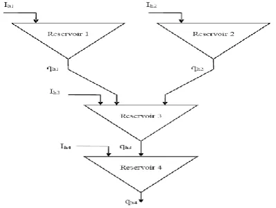
algorithm. The effect of valve point loading has been taken into consideration to illustrate the robustness of the proposed method. The transport time delay between cascaded reservoirs is also considered in this case study. The scheduling time period is one day with 24 intervals of one hour each. The data of test system are taken from [16]. The configuration of multi chain hydro sub system is shown in “Fig. 2”. The water time transport delays between connected reservoirs are given in Table 1.

The hydro power generation coefficients are given in Table 2. The reservoir storage limits, discharge rate limits, initial and final reservoir storage volume conditions and the generation limits of hydro power plants are shown in Table 3. Table 4 shows the reservoir inflows of hydro power plants. The fuel cost coefficients and power output limits of thermal units are given in Table 5. The load demand over the 24 hours is given in Table 6. The control parameters of ABC algorithm are given in Table 7.

The optimal solution obtained from ABC algorithm is achieved in 50 trial runs. The optimal hourly hydrothermal generation schedule and hourly total fuel cost obtained by the ABC algorithm is shown in Table 8. Table 9 shows the optimal hourly water discharge of hydro power plants obtained from the ABC algorithm while Table 10 presents the optimal hourly storage volumes of hydro reservoirs obtained from the ABC algorithm.

The proposed algorithm has been implemented in MATLAB language and executed on an Intel Core i3, 2.27 GHz personal computer with a 3.0 GB of RAM.

Figure 2: Multi chain hydro sub system networks

TABLEI

WATER TIME TRANSPORT DELAYS BETWEEN CONNECTED RESERVOIRS

Plant 1 2 3 4

Ru 0 0 2 1

τu 2 3 4 0

Ru : Number of upstream hydro power plants τu : Time delay to immediate downstream hydro power plant

TABLEII

HYDRO POWER GENERATION COEFFICIENTS

Plant C1 C2 C3 C4 C5 C6

1 -0.0042 -0.4200 000300 0.9000 100000 -50.000

2 -0.0040 -0.3000 0.0150 101400 905000 -70.000

3 -0.0016 -0.3000 000140 005500 505000 -40.000

4 -0.0030 -0.3100 000270 104400 140000 -90.000 TABLEIII

RESERVOIR STORAGE CAPACITY LIMITS, PLANT DISCHARGE LIMITS, PLANT GENERATION LIMITS AND RESERVOIR END

CONDITIONS (×10 m4 3₎

Plant V_hmin V_hmax V_hini V_hend qmin_h qmax_h P_hmin P_hmax

1 80 150 100 120 5 15 0 500

2 60 120 80 70 6 15 0 500

3 100 240 170 170 10 30 0 500

4 70 160 120 140 13 25 0 500

TABLEIIV

RESERVOIR INFLOWS OF MULTI CHAIN HYDRO PLANTS (_{×10 m}4 3₎

Hour Reservoir Hour Reservoir

1 2 3 4 1 2 3 4

1 10 8 801 208 13 11 8 4 0

2 9 8 802 204 14 12 9 3 0

3 8 9 4 106 15 11 9 3 0

4 7 9 2 0 16 10 8 2 0

5 6 8 3 0 17 9 7 2 0

6 7 7 4 0 18 8 6 2 0

7 8 6 3 0 19 7 7 1 0

8 9 7 2 0 20 6 8 1 0

9 10 8 1 0 21 7 9 2 0

10 11 9 1 0 22 8 9 2 0

11 12 9 1 0 23 9 8 1 0

12 10 8 2 0 24 10 8 0 0

TABLEV

FUEL COST COEFFICIENTS AND OPERATING LIMITS OF THERMAL UNITS

Unit ai bi ci ei fi min gi

P P_gimax

TABLEVIII LOAD DEMAND FOR 24 HOUR

Hour PD

(MW) Hour PD

(MW) Hour PD

(MW) Hour PD

(MW)

1 750 7 950 13 1110 19 1070

2 780 8 1010 14 1030 20 1050

3 700 9 1090 15 1010 21 910

4 650 10 1080 16 1060 22 860

5 670 11 1100 17 1050 23 850

6 800 12 1150 18 1120 24 800

TABLEVII

CONTROL PARAMETERS OF ABC ALGORITHM

ABC algorithm parameters Value

Colony size (Np) 50

Number of food sources (Ns) 25 Number of employed bees 25

Number of onlookers 25

Maximum cycle number (MCN) 300

Limit value 100

TABLEVIII

HOURLY OPTIMAL HYDROTHERMAL GENERATION SCHEDULE USING ABC ALGORITHM

Hour Thermal generation (MW) Hydro generation (MW)

Total fuel cost ($/hr)

Pg1 Pg2 Pg3 Ph1 Ph2 Ph3 Ph4

1 102.4411 18102670 5000000 7305131 6205056 5308689 22604043 1353.8 32 2 2201315 12605600 17402240 9500352 5507258 4200007 26403229 1356.6

46 3 4600797 13302205 14007144 5506823 6703702 0000000 25609329 1332.4

92 4 2000000 11509043 8601655 6807149 8201708 3906308 23704138 1143.5

26 5 15703638 4000000 5000000 9001544 7509778 0000000 25605040 1128.2

46 6 11201576 4608703 22604150 6909569 5806992 4602835 23906174 1446.5

62 7 6508606 20907137 23004331 5201114 7406900 4706980 26904933 1795.3

53 8 12903525 21107074 23100256 6806976 4602139 3906663 28303367 1967.1

27 9 10302970 21000890 35209299 5905113 5806124 5104951 25400652 2285.7

79 10 10308887 21400891 31102150 6409068 6505284 2402415 29601305 2070.2

65 11 11209518 21207889 32200855 8501607 4303682 5304024 27002423 2133.2

67 12 10202374 29405060 32402013 8001515 3906928 5307267 25504843 2279.8

80 13 17409917 28905292 22900650 8903898 4805825 4900964 22903454 2249.6

67 14 10101384 29307887 21206150 9207409 4307653 5401977 23107539 2039.3

67 15 4501796 21006628 32003588 9601910 5304461 5308540 23003078 1986.9

27 16 12700743 21000301 31903423 5500720 6409931 5602501 22702381 2185.5

42 17 17309267 20809086 22709670 8505090 4908735 5603430 24704722 2001.5

96 18 17200041 29304674 22901950 9805474 3909007 5900776 22708078 2242.3

14 19 10004064 20709049 31700150 8109545 4509833 4007904 27509455 2012.4

54 20 17500000 20808229 22900754 6105574 4608905 4606797 28109741 1994.3

70 21 2500439 21001011 23001837 7405008 5809527 5408876 25603302 1563.5

78 22 7600859 12403536 22902102 6800906 5206797 5305424 25600375 1568.8

47 23 2000000 14700406 23003625 9903709 4709393 5806357 24606510 1482.9

69 24 10303851 12602126 14006553 6608475 5001730 5700228 25507036 1289.1

94

TABLEIX

HOURLY HYDRO PLANT DISCHARGE USING ABC ALGORITHM

Hour Hydro plant discharges (×10 m /hr4 3 )

qh1 qh2 qh3 qh4

1 706477 800963 1603437 1400836 2 1208578 608962 1902194 1809513 3 503388 808177 2506760 1600064 4 609983 1300735 1508037 1304801 5 1105135 1200182 2409377 1404783 6 704305 803711 1104678 1300000 7 500000 1407109 1005282 1702684 8 700322 703416 1800360 1907492 9 507130 1000189 1404034 1506409 10 602676 1109777 2108457 2304767 11 901414 609553 1206409 1903910 12 802567 601849 1307150 1707008 13 907922 705317 1700259 1308451 14 1003885 604754 1503728 1309507 15 1101753 709140 1600444 1305071 16 500000 1006610 1407236 1300000 17 808969 707224 1503980 1502572 18 1106836 601585 1304430 1300000 19 804627 701085 2009065 1808872 20 507406 700701 1903231 2001202 21 703458 900879 1607212 1600635 22 604966 707739 1705217 1507994 23 1200324 608722 1409395 1406374 24 603383 701300 1507040 1507211

TABLEX

HOURLY STORAGE VOLUME OF HYDRO RESERVOIRS USING ABC ALGORITHM

Hour Reservoir storage volume ( 4 3

×10 m )

Vh1 Vh2 Vh3 Vh4

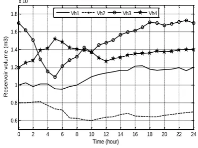
In order to verify and validate the effectiveness of the proposed algorithm, its simulation results will be compared with those obtained from the SA, EP, GA and CFPSO technique. Table 11 shows the comparison of total fuel cost and execution time of the proposed algorithm among other methods. From Table 11, it is clear that the ABC algorithm performs better than SA, EP, GA and CFPSO technique in terms of total fuel cost and execution time. “Fig. 3” shows the hourly thermal plant power generation by using proposed method, the hourly hydro plant power generation by using proposed algorithm is given in “Fig. 4”, the hourly hydro plant discharges using ABC algorithm are shown in “Fig. 5” and “Fig. 6” presents the hourly reservoir storage volumes using proposed technique.

TABLEXI

COMPARISON OF TOTAL FUEL COST AND COMPUTATION TIME OF THE

PROPOSED TECHNIQUE AMONG SA,EP,GA AND CFPSO METHODS

Method Total fuel cost ($) CPU Time (Sec)

ABC 42909.009 79.16

SA [22] 45466.000 246.19

EP [22] 47306.000 9879.45

CFPSO [23] 44925.620 183.64

GA [23] 45392.009 198.57

2 4 6 8 10 12 14 16 18 20 22 24 0

100 200 300 400 500 600 700 800 900

Time (hour)

T

h

e

rm

a

l

g

e

n

e

ra

ti

o

m

(

M

W

)

Pth Pg1 Pg2 Pg3

Figure 3: Hourly thermal plant power generation using ABC algorithm

2 4 6 8 10 12 14 16 18 20 22 24 0

50 100 150 200 250 300 350 400 450 500 550

Time (Hour)

H

yd

ro

g

e

n

e

ra

ti

o

n

(

M

W

)

Ph Ph1 Ph2 Ph3 Ph4

Figure 4: Hourly hydro plant power generation using ABC algorithm

2 4 6 8 10 12 14 16 18 20 22 24 0.5

1 1.5 2 2.5

3x 10

5

Time (Hour)

H

yd

ro

d

isc

h

a

rg

e

(

m

3

/h

r)

qh1 qh2 qh3 qh4

Figure 5: Hourly hydro plant discharges using ABC algorithm

0 2 4 6 8 10 12 14 16 18 20 22 24 0.6

0.8 1 1.2 1.4 1.6 1.8

x 106

Time (hour)

R

e

se

rvo

ir

vo

lu

m

e

(

m

3

)

Vh1 Vh2 Vh3 Vh4

Figure 6: Hourly hydro reservoir storage volumes using ABC algorithm

VII.

CONCLUSION

In this paper, an artificial bee colony (ABC) algorithm has been developed to solve the short term hydrothermal generation scheduling problem. To demonstrate the feasibility and performance efficiency of the proposed algorithm, a multi chain hydrothermal system was tested. The effect of valve point loading is considered in this case study to verify the robustness of the proposed technique. The numerical results indicate that the ABC algorithm can obtain better schedule results with minimum generation cost and lower execution time when compared with other evolutionary algorithms such as SA, EP, GA and CFPSO technique.

VIII.

REFERENCES

[1] A.J. Wood and B.F. Wollenberg, "Power Generation, Operation, and Control", John Wiley and Sons., New York, 1984.

[2] D.P. Kothari and J.S. Dhillon, "Power system optimization", New Delhi, India, Pvt. Ltd, 2009.

problem", Electric Power System Research, vol. 79, pp. 1308-1320, 2009

[4] J. Tang and P.B. Luh, "Hydro thermal scheduling via extended differential dynamic programming and mixed coordination", IEEE Trans. Power Syst., vol. 10, no. 4 pp. 2021-2028, Nov.,1995.

[5] Y. Jin-Shyr and C. Nanming, "Short term hydro thermal coordination using multi pass dynamic programming", IEEE Trans. Power Syst., vol. 4, pp. 1050-1056, 1989.

[6] X. Guan, E. Ni, R. Li and P.B. Luh, " An optimization based algorithm for scheduling hydro thermal power systems with cascaded reservoirs and discrete hydro constraints", IEEE Trans. Power Syst., vol. 12, pp. 1775-1780, 1997.

[7] S. Al-Agtash, "Hydro thermal scheduling by augmented lagrangian: consideration of transmission constraints and pumped storage units", Power Engineering Review, IEEE, vol. 21, pp. 58-59, 2001.

[8] O. Nilsson and D. Sjelvgren, "Mixed integer programming applied to short term planning of a hydro thermal system", IEEE Trans. Power Syst., vol. 11, pp. 281-286, 1996. [9] L.M. Kimball, K.A. Clements, P.W. Davis and I. Nejdawi,

"Multi period hydro thermal economic dispatch by an interior point method", Mathematical Problems in Engineering, vol. 8, pp. 33-42, 2002.

[10] J. Maturana, M-C. Riff," Solving the short-term electrical generation scheduling problem by an adaptive evolutionary approach", European Journal of Operational Research, vol. 179, pp. 677-691, 2007.

[11] N.C. Nayak and C.C.A. Rajan, "Hydro thermal scheduling by an evolutionary programming method with cooling-banking constraints", International Journal of Soft Computing and Engineering (IJSCE), Issue .3, vol. 2, pp. 517-521, July, 2012. [12] D.P. Wong and Y.W. Wong, "Short term hydro thermal scheduling part. I. Simulated annealing approach", Generation, Transmission and Distribution, IEE Proceeding, vol. 141, pp. 497-501, 1994.

[13] D.N. Simopoulos, S.D. Kavatza and C.D. Vournas, "An enhanced peak shaving method for short term hydro thermal scheduling", Energy Conversion and Management, vol. 48, pp. 3018-3024, 2007.

[14] T. Jayabarathi, S. Chalasani and Z.A. Shaik, "Hybrid differential evolution and particle swarm optimization based solutions to short term hydro thermal scheduling", WSEAS Trans. Power Syst., Issue 11, vol. 2, Nov.,2007.

[15] V.N. Diew and W. Ongsakul, "Enhanced merit order and augmented lagrange Hopfield network for hydro thermal scheduling", International Journal of Electrical Power & Energy Systems, vol. 30, no. 2, pp. 93-101, 2008.

[16] M. Basu, "An interactive fuzzy satisfying method based on evolutionary programming technique for multi objective short-term hydro thermal scheduling", Electric Power Systems Research, vol. 69, pp. 277-285, 2004.

[17] E. Gil, J. Bustos, H. Rudnick," Short term hydrothermal generation scheduling model using genetic algorithm", IEEE Trans. Power Syst. vol. 18, no. 4, pp. 1256-1264, Nov., 2003.

[18] C.E. Zoumas, A.G. Bakirtzis, J.B. Theocharis, V. Petridis," A genetic algorithm solution approach to the hydro thermal coordination problem", IEEE Trans. Power Syst., vol. 19, no. 2, pp. 1356-1364, May, 2004.

[19] A. George, M.C. Reddy and A.Y. Sivaramakrishnan, "Short term hydro thermal scheduling based on multi-objective genetic algorithm", International Journal of Electrical Engineering, vol. 3, no. 1, pp. 13-26, 2010.

[20] G. Sreenivasan, C.H. Saibabu, S. Sivanagaraju," PSO based short-term hydrothermal scheduling with prohibited discharge zones", International Journal of Advanced Computer Science and Applications, vol. 2, no. 9, pp. 97-105, 2011.

[21] C. Sun and S. Lu, "Short term combined economic emission hydro thermal scheduling using improved quantum-behaved particle swarm optimization", Expert Syst. App., vol. 37, pp. 4232-4241, 2010.

[22] K.K. Mandal, M. Basu and N. Chakraborty, "Particle swarm optimization technique based short-term hydrothermal scheduling", Applied Soft Computing, pp. 1392-1399,2008. [23] M.M. Salama, M.M. Elgazar, S.M. Abdelmaksoud and H.A.

Henry, "Optimal generation scheduling of cascaded hydrothermal system using genetic algorithm and constriction factor based particle swarm optimization technique", International Journal of Scientific and Engineering Research, vol. 4, Issue 5, pp. 750-761, May, 2013.

[24] I.A. Farhat and M.E. El-Hawary, "Short-term hydro-thermal scheduling using an improved bacterial foraging algorithm", IEEE Electrical Power & Energy Conference, pp. 1-5, 2009. [25] D. Karaboga and B. Akay, "A comparative study of artificial

bee colony algorithm", Applied Mathematics and Computation, vol. 214 pp. 108-132, 2009.

[26] H.A. Shayanfar, E.S. Barazandeh, S.J. Seyed Shenava, A. Ghasemi and O. Abedinia, "A Solving optimal unit commitment by improved honey bee mating optimization", international Journal on Technical and Physical Problems of Engineering, vol. 4, no.4 pp. 38-45, Dec., 2012.