University of Pennsylvania
ScholarlyCommons
Publicly Accessible Penn Dissertations
1-1-2015
VIVA: An Online Algorithm for Piecewise Curve
Estimation Using ℓ
0
Norm Regularization
Richard Benjamin Voigt
University of Pennsylvania, [email protected]
Follow this and additional works at:
http://repository.upenn.edu/edissertations
Part of the
Applied Mathematics Commons
,
Electrical and Electronics Commons
, and the
Operational Research Commons
This paper is posted at ScholarlyCommons.http://repository.upenn.edu/edissertations/1158 For more information, please [email protected].
Recommended Citation
Voigt, Richard Benjamin, "VIVA: An Online Algorithm for Piecewise Curve Estimation Using ℓ0Norm Regularization" (2015). Publicly Accessible Penn Dissertations. 1158.
VIVA: An Online Algorithm for Piecewise Curve Estimation Using ℓ
0
Norm Regularization
Abstract
Many processes deal with piecewise input functions, which occur naturally as a result of digital commands,
user interfaces requiring a confirmation action, or discrete-time sampling. Examples include the assembly of
protein polymers and hourly adjustments to the infusion rate of IV fluids during treatment of burn victims.
Estimation of the input is straightforward regression when the observer has access to the timing information.
More work is needed if the input can change at unknown times. Successful recovery of the change timing is
largely dependent on the choice of cost function minimized during parameter estimation.
Optimal estimation of a piecewise input will often proceed by minimization of a cost function which includes
an estimation error term (most commonly mean square error) and the number (cardinality) of input changes
(number of commands). Because the cardinality (ℓ
0norm) is not convex, the ℓ
2norm (quadratic smoothing)
and ℓ
1norm (total variation minimization) are often substituted because they permit the use of convex
optimization algorithms. However, these penalize the magnitude of input changes and therefore bias the
piecewise estimates. Another disadvantage is that global optimization methods must be run after the end of
data collection.
One approach to unbiasing the piecewise parameter fits would include application of total variation
minimization to recover timing, followed by piecewise parameter fitting. Another method is presented herein:
a dynamic programming approach which iteratively develops populations of candidate estimates of increasing
length, pruning those proven to be dominated. Because the usage of input data is entirely causal, the algorithm
recovers timing and parameter values online. A functional definition of the algorithm, which is an extension of
Viterbi decoding and integrates the pruning concept from branch-and-bound, is presented. Modifications are
introduced to improve handling of non-uniform sampling, non-uniform confidence, and burst errors.
Performance tests using synthesized data sets as well as volume data from a research system recording fluid
infusions show five-fold (piecewise-constant data) and 20-fold (piecewise-linear data) reduction in error
compared to total variation minimization, along with improved sparsity and reduced sensitivity to the
regularization parameter. Algorithmic complexity and delay are also considered.
Degree Type
Dissertation
Degree Name
Doctor of Philosophy (PhD)
Graduate Group
Electrical & Systems Engineering
First Advisor
Jonathan M. Smith
Keywords
changepoint, curve fitting, denoising, joinpoint, regression, regularization
Subject Categories
Applied Mathematics | Electrical and Electronics | Operational Research
VIVA: AN ONLINE ALGORITHM FOR PIECEWISE CURVE ESTIMATION
USING`0 NORM REGULARIZATION
Richard B. Voigt
A DISSERTATION
in
Electrical and Systems Engineering
Presented to the Faculties of the University of Pennsylvania
in
Partial Fulfillment of the Requirements for the
Degree of Doctor of Philosophy
2015
Supervisor of Dissertation
Jonathan M. Smith
Olga and Alberico Pompa Professor of Engineering and Applied Science
Graduate Group Chairwoman
Saswati Sarkar
Professor, Electrical and Systems Engineering
Dissertation Committee
Ali Jadbabaie, Alfred Fitler Moore Professor of Network Science, Electrical and Systems Engi-neering
Jonathan M. Smith, Olga and Alberico Pompa Professor of Engineering and Applied Science, Computer and Information Science
Saleem Kassam, Solomon and Sylvia Charp Professor, Electrical and Systems Engineering Insup Lee, Cecilia Fitler Moore Professor, Computer and Information Science
VIVA: AN ONLINE ALGORITHM FOR PIECEWISE CURVE ESTIMATION
USING`0 NORM REGULARIZATION
COPYRIGHT
© 2015
iii
Acknowledgements
Doctoral work is not performed in a vacuum (after all, even the mighty doctoral student is not immune to asphyxiation), and mine has been no exception to that rule. I count many blessings bestowed by the providential hand of a great God and His Son, the Lord Jesus Christ – loving family and friends, innate abilities and the professors and colleagues in university and industry who developed them, opportunities to use them – these have been no less essential to my journey than breath itself. To name each individual who has guided, advised, encouraged, or otherwise assisted me would eclipse any dissertation... and my memory is not up to the task in any case. Nevertheless, I would like to offer special thanks to several who stand out.
From the very beginning I have been influenced by my mother Dr. Mary Voigt (PhD), who taught me mathematics, reading, scientific methods, to always look for ulterior motives, and that skepticism and understanding one’s relationship to God are not mutually exclusive and my father Richard H. Voigt, who has never let me forget that honorifics and intelligence are worth nothing without honor and integrity. I thank them for their unceasing love and all the ways they’ve showed it. And if my grandparents and siblings have shown me less love, it is only in degree and not in kind.
I thank my elementary and high school teachers for teaching me, as much about the expec-tations of society as about the course topics, and particularly for a lesson in Pre-Calculus about using extraordinary gifts to help those around me instead of alienating them (although it took me a few more years to achieve passing competence). KSU EECE professors William Kuhn, PhD and Don Gruenbacher, PhD, thank you for a first taste of engineering research, via poster presentations hung on the walls of Rathbone Hall, and thanks to James DeVault, PhD and An-drew Rys, PhD who convinced me to apply for graduate fellowships so I could perform research myself. Also to Mr. George Beck and KSU professors Medhat Morcos, PhD and Steve War-ren, PhD for seeing more potential in me than I could in myself... and whose recommendations swayed the NDSEG fellowship and Penn admissions committees to agree. NASA flight surgeon Dr. Douglas Hamilton, MD I thank for getting me interested in medical data and devices and teaching me everything I know about cardiology (and Canada), in addition to no small amount of personal mentoring. Drs. Don Hummels (PhD) and Russ Meier (PhD) I credit with focusing me on practical engineering and real-time signal processing, and then Penn ESE professors Ali Jadbabaie, PhD, George Pappas, PhD, and Srisankar Kunniyur, PhD took those tools to the next level by adding a theoretic framework. Also Dr. Santosh Venkatesh (PhD), who installed a healthy fear and awe of mathematics that most of my peers had acquired much earlier, and whom I will never, ever bet against.
ACKNOWLEDGEMENTS iv
sinking into despair as I dealt with the disintegration of a particularly important personal rela-tionship, and helped me prioritize. Coworkers at Wyle, UTMB, and Sparx helped me maintain balance while juggling work, school, church, and personal issues, backfilled for me when I needed a more intense focus on academic work, and most recently courageously served, without pay, as proofreaders.
Dr. George Kramer (PhD), professor of anesthesiology and director of the Resuscitation Research Lab at UTMB, thank you for correcting all my prior misconceptions about what re-search is (or at least, replacing them with your own), welcoming me into a medical rere-search environment and freely sharing project ideas and data, supporting conference travel and poster presentations, introducing me to world-famous scientists, showing your dedication to personal leadership through sharing proverb after (often completely fabricated and usually inappropriate) anecdote, and always, ALWAYS being willing to buy me more beers than I was willing to drink.
To the other students of the Penn CIS Distributed Systems Laboratory, for fitting me into your presentation schedule, listening to several half-baked and wholly disorganized slide sets over the years, and always making me feel welcome, thank you. To all the researchers of the UTMB Resuscitation Research Lab, postdocs, technicians, nurses, and staff anesthesiologists alike, I am indebted for your efforts to put those half-baked ideas into practice in animal surgeries and collect the data I requested, for enduring my total misconceptions about physiology and carefully (and oh-so-patiently) setting me straight over many months, and for the friendships that grew.
I would also like to thank the LATEX developers, the MiKTeX package maintainers, the tex.stackexchange.com community, and especially Dr. Christian Feuers¨anger for his pgfplots package, without which this document would be far less attractive. A gift of Visual Studio from the Microsoft MVP program has also been most helpful.
Finally, and most important, my advisor, dissertation supervisor, and friend, Dr. Jonathan Smith (PhD), who taught me the art of turning priorities into actions, explained the brotherhood of PhD engineers in terms even I could understand, gave invaluable feedback and direction on this entire undertaking and kept me on track across more than a decade despite my inadequacies and competing demands, deserves more thanks than I can express.
My successes I owe to all those named above as well as others who have labored without recognition; mistakes and omissions are my own.
I also acknowledge the following sources of funding which made possible my doctoral studies, research experiments which generated data for my use, and my analysis:
• National Defense Science and Engineering Graduate Fellowship, award years 2002-2005
• National Science Foundation, grant CNS-1040672 “FIA: NEBULA“
• Olga and Aberico Pompa Professorship, an endowed chair at the University of Penn-sylvania
• Office of Naval Research, grant N00014-12-C-0556 “Decision Support and Closed Loop Control Systems”
• U.S. Army Medical Research and Materiel Command, Cooperative Agreement #09078006 “Titrated Bolus Resuscitation“
• National Institutes of Health, grant 1R01HL092253-01 “Decision-Assist and Closed-Loop Resuscitation of Burn-Injured Patients”
v
ABSTRACT
VIVA: AN ONLINE ALGORITHM FOR PIECEWISE CURVE ESTIMATION
USING`0 NORM REGULARIZATION
Richard B. Voigt
Jonathan M. Smith
Many processes deal with piecewise input functions, which occur naturally as a result of digital commands, user
interfaces requiring a confirmation action, or discrete-time sampling. Examples include the assembly of protein
polymers and hourly adjustments to the infusion rate of IV fluids during treatment of burn victims. Estimation
of the input is straightforward regression when the observer has access to the timing information. More work is
needed if the input can change at unknown times. Successful recovery of the change timing is largely dependent
on the choice of cost function minimized during parameter estimation.
Optimal estimation of a piecewise input will often proceed by minimization of a cost function which includes
an estimation error term (most commonly mean square error) and the number (cardinality) of input changes
(number of commands). Because the cardinality (`0norm) is not convex, the`2norm (quadratic smoothing) and
`1norm (total variation minimization) are often substituted because they permit the use of convex optimization
algorithms. However, these penalize the magnitude of input changes and therefore bias the piecewise estimates.
Another disadvantage is that global optimization methods must be run after the end of data collection.
One approach to unbiasing the piecewise parameter fits would include application of total variation minimization
to recover timing, followed by piecewise parameter fitting. Another method is presented herein: a dynamic
programming approach which iteratively develops populations of candidate estimates of increasing length, pruning
those proven to be dominated. Because the usage of input data is entirely causal, the algorithm recovers timing
and parameter values online. A functional definition of the algorithm, which is an extension of Viterbi decoding
and integrates the pruning concept from branch-and-bound, is presented. Modifications are introduced to improve
handling of non-uniform sampling, non-uniform confidence, and burst errors. Performance tests using synthesized
data sets as well as volume data from a research system recording fluid infusions show five-fold (piecewise-constant
data) and 20-fold (piecewise-linear data) reduction in error compared to total variation minimization, along with
improved sparsity and reduced sensitivity to the regularization parameter. Algorithmic complexity and delay are
vi
Contents
Acknowledgements iii
Abstract v
List of Tables ix
List of Illustrations x
Chapter 1. Background 1
1.1. The Value of Infusion Monitoring 1
1.2. Practical Measurement of Infusion Rate 4
1.3. Existing Methods for Denoising Piecewise Signals 5
1.3.1. Bicriterion Model 5
1.3.2. Inexact Methods 6
1.3.3. Convex Methods 6
1.3.4. Equivalent Mixed-Integer Models 9
1.3.5. Methods of Solving Integer Programs 10
1.3.6. Related Work in Dynamic Programming 12
1.4. Real-Time Implications 14
Chapter 2. Short History of the Project 15
Chapter 3. Piecewise Minimum Cardinality Curve Fitting
using Pruned Dynamic Programming 17
3.1. Optimality Criterion for Continuity-Constrained Piecewise Curve Fitting 17
3.2. Complexity Growth in Small Cases 20
3.3. Functional Description of VIVA Algorithm 23
3.4. Truncated Search Heuristics 24
3.4.1. “Freeze Old Segments” Heuristic 25
3.4.2. “Limited Branching” Heuristic 26
3.5. Case Study, Compression of Electrocardiogram Data 27
3.6. Evaluation of Signal Recovery Performance using Synthesized Data 29
3.6.1. Monte-Carlo Testing Methodology 29
3.6.2. Piecewise Constant 30
3.6.3. Piecewise Linear 32
Chapter 4. Confidence Weighting 36
4.1. Measurement Variance 36
4.1.1. Inclusion of Weighting Term in Bicriterion Regularization 37
CONTENTS vii
4.2. Burst Noise and Denoising Performance 38
4.2.1. Unweighted Estimator Performance Degradation due to Burst Noise 40
4.2.2. Variance-Based Weighting Provides Robustness to Burst Noise 41
4.2.3. Impact of Variance-Based Weighting on Strictly White Noise 51
4.2.4. Spectrum of residual noise 56
4.3. Case Study, Load Cell Monitoring Resuscitation of Hemorrhagic Shock 57
Chapter 5. Error and Delay in Online Configurations 61
5.1. Zero-Delay Evaluation 61
5.2. Changepoint Detection Lag 62
5.2.1. Solution Stability Condition 62
5.2.2. Selecting Delay Based on Solution Stability 64
5.2.3. Selecting Delay Based on Observed Population Reduction 65
5.3. Online Denoising Performance 65
5.3.1. Piecewise-constant with additive i.i.d. Gaussian noise 65
5.3.2. Piecewise-constant with burst Gaussian noise 65
5.3.3. Piecewise-linear with i.i.d. Gaussian noise 66
5.3.4. Piecewise-linear with burst white Gaussian noise 66
Chapter 6. Conclusions 74
6.1. Summary 74
6.2. Impact 74
6.3. Whither? 75
Appendix A. SelectedMatlaband C# Functions 76
A.1. Synthesis of test data for Monte Carlo analysis 76
A.1.1. gen piecewise constant.m 76
A.1.2. gen piecewise linear.m 77
A.1.3. gen iid white noise.m 77
A.1.4. gen burst white noise.m 78
A.2. Optimality Testing 79
A.2.1. Connected Piecewise-Linear Regression (Polyline fitting) 79
A.3. VIVA Implementation 81
A.3.1. Piecewise-Constant State Update and Branch 81
A.3.2. Piecewise-Linear State Update and Branch 84
A.3.3. Pruned Depth-First Search 90
Appendix B. Solutions to Least-Squares Subproblems 97
B.1. Minimum-Residual Constant Segment Estimate 97
B.1.1. Least-Squares Solution 97
B.1.2. Residual Error 98
B.2. Minimum-Residual Polyline Estimate 99
B.2.1. Least-Squares Solution 99
Appendix C. Summary of measurement statistics 104
C.1. Continuous time 104
C.1.1. Recursive update 104
CONTENTS viii
C.2. Discrete time 105
C.2.1. Recursive Update 105
Appendix D. Linear Relaxations 106
Appendix E. Small Polyline fitting examples 108
ix
List of Tables
1 Comparison of residual error and sparsity of trend-filter estimates 8
2 Residual error and optimality, by segment count, for the S&P 500 log(price) excerpt
polyline approximations 22
3 Heuristics’ Influence on ECG Polyline Approximation (Compression) Performance 29
A.1 Size of Monte Carlo datasets 76
E.1 Residual error and bicriterion-optimality, by segment count, for the noiseless “sloop”
polyline approximations of Figure E.2 109
E.2 Residual error and bicriterion-optimality, by segment count, for the “sloop with
measurement noise” polyline approximations of Figure E.5 111
E.3 Residual error and bicriterion-optimality, by segment count, for the noiseless “gaff
cutter” polyline approximations of Figure E.9 114
E.4 Residual error and optimality, by segment count, for the noisy “gaff cutter” signal
x
List of Illustrations
1 In Total Variation Minimization, the penalty function biases the estimate for
extreme segments 7
2 Stairsteps form in Total Variation Minimization, because the penalty function
assigns zero incremental cost to segments which lie between neighbors 7
3 `1 Trend Filter is systematically biased toward shallow changes in slope 8
4 The binary sequencebj segments the measurement sequence yj into independent
constant segments 9
5 Cancel common term, yielding necessary condition for prefix of optimal segmentation 19
6 Exact polyline search algorithms’ complexity, considering first 600 data of S&P 500
log(price) data (Little and Jones, 2010) 21
7 Optimal polyline approximations for first 600 samples of S&P 500 log(price) data
(Little and Jones, 2010) 22
8 Model of many conjoined piecewise-linear segments 25
9 Model of many conjoined piecewise-linear segments with segment freeze heuristic 26
10 Excerpt of ECG data compression example data, with vertical offset added for ease
of comparison 27
11 Close zoom into ECG data compression example data 28
12 The signal piecewise constant.mat with and without noise 30
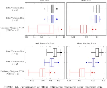
13 Performance of offline estimators evaluated using piecewise constant signal (strongly
white noise), N = 240 31
14 Performance in stable regions (transition bands excluded) of offline estimators evaluated using piecewise constant signal (strongly white noise), N = 240 31
15 Sparsity using Pruned Dynamic Programming on Piecewise Constant Signal 32
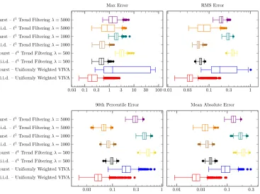
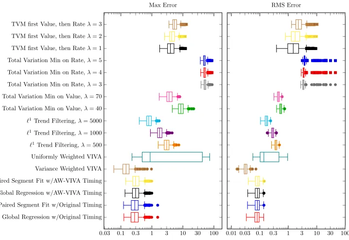
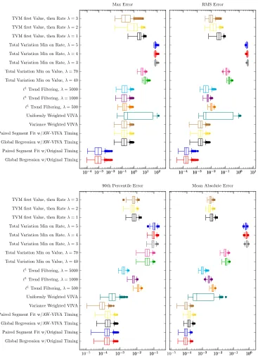
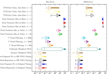
16 Performance of offline estimators evaluated using piecewise linear signal (strongly
white noise), N = 500, analysis of value estimate 33
17 Performance in stable regions (transition bands excluded) of offline estimators evaluated using piecewise linear signal (strongly white noise), N = 500, analysis of
value estimate 33
18 Performance of offline estimators evaluated using piecewise linear signal (strongly
white noise), N = 500, analysis of rate estimate 34
19 Performance in stable regions (transition bands excluded) of offline estimators evaluated using piecewise constant signal (strongly white noise), N = 500, analysis
of rate estimate 34
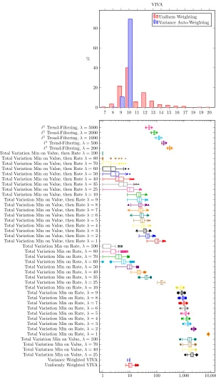
20 Comparison of Sparsity Achieved by all offline methods with piecewise linear signal
LIST OF ILLUSTRATIONS xi
21 The signal piecewise constant bursty.mat with and without noise 38
22 “Transmitted” Signal 39
23 “Received” Signal corrupted by burst noise 39
24 Performance degradation of offline estimators when burst noise is introduced into
piecewise constant signal 40
25 Performance degradation in stable regions (transition bands excluded) of offline estimators when burst noise is introduced into piecewise constant signal 40
26 Effect of Burst Noise on Estimate Sparsity 41
27 Performance degradation of offline value estimates when burst noise is introduced
into piecewise linear signal 42
28 Performance degradation in stable regions (transition bands excluded) of offline value estimates when burst noise is introduced into piecewise linear signal 42
29 Performance degradation of offline rate estimates when burst noise is introduced
into piecewise linear signal 43
30 Performance degradation in stable regions (transition bands excluded) of offline rate estimates when burst noise is introduced into piecewise linear signal 43
31 Performance of offline estimators evaluated using piecewise constant signal (burst
noise), N = 100 44
32 Performance in stable regions (transition bands excluded) of offline estimators
evaluated using piecewise constant signal (burst noise), N = 100 44
33 Sparsity achieved by offline estimators evaluated using piecewise constant signal
(burst noise), N = 100 45
34 Performance of offline estimators evaluated using piecewise linear signal (burst
noise), N = 500, analysis of value estimate 46
35 Performance in stable regions (transition bands excluded) of offline estimators evaluated using piecewise linear signal (burst noise), N = 500, analysis of value
estimate 47
36 Performance of offline estimators evaluated using piecewise linear signal (burst
noise), N = 500, analysis of rate estimate 48
37 Performance in stable regions (transition bands excluded) of offline estimators evaluated using piecewise linear signal (burst noise), N = 500, analysis of rate
estimate 49
38 Comparison of Sparsity Achieved by all offline methods with piecewise linear signal
(burst noise), N=500 50
39 Performance of offline estimators evaluated using piecewise constant signal (strongly
white noise), N = 240 51
40 Performance in stable regions (transition bands excluded) of offline estimators evaluated using piecewise constant signal (strongly white noise), N = 240 51
41 Sparsity achieved by offline estimators evaluated using piecewise constant signal
(strongly white noise), N = 240 52
42 Performance of offline estimators evaluated using piecewise linear signal (strongly
white noise), N = 500, analysis of value estimate 53
43 Performance in stable regions (transition bands excluded) of offline estimators evaluated using piecewise linear signal (strongly white noise), N = 500, analysis of
LIST OF ILLUSTRATIONS xii
44 Performance of offline estimators evaluated using piecewise linear signal (strongly
white noise), N = 500, analysis of rate estimate 54
45 Performance in stable regions (transition bands excluded) of offline estimators evaluated using piecewise constant signal (strongly white noise), N = 500, analysis
of rate estimate 54
46 The signalpiecewise linear.matwith and without noise 55
47 Signal corrupted by sporadic noise and recovered using inverse-variance
auto-weighting 56
48 Sporadic noise and residual error after recovery using inverse-variance auto-weighting 56
49 Power spectral density of sporadic noise and residual error 57
50 Load cell data monitoring pig hemorrhage and resuscitation 58
51 Piecewise linear estimate obtained to denoise load cell channel 2, Figure 50 59
52 Flow rates obtained from piecewise linear estimate 60
53 Total flow rate from multiple load cells, comparison to electronic Doppler flowmeter 60
54 Excerpt from ’piecewise constant.mat’ and corresponding zero-delay estimate
(Uniformly weighted,ζ= 25) 61
55 Excerpt from ’piecewise linear bursty.mat’ and corresponding zero-delay
estimate (Variance auto-weighted,ζ= 25) 62
56 Cost function withinbk= 0 branch 63
57 Cost function withinbk= 1 branch 64
58 Denoising piecewise constant.mat using conventional lowpass filters and VIVA 66
59 Performance of online estimators evaluated using piecewise constant signal (strongly
white noise), N = 240 67
60 Performance in stable regions (transition bands excluded) of online estimators evaluated using piecewise constant signal (strongly white noise), N = 240 67
61 Denoising piecewise constant bursty.mat using conventional lowpass filters and
Variance Auto-Weighted VIVA 68
62 Performance of online estimators evaluated using piecewise constant signal (burst
noise), N = 100 69
63 Performance in stable regions (transition bands excluded) of online estimators
evaluated using piecewise constant signal (burst noise), N = 100 69
64 Performance of online estimators evaluated using piecewise linear signal (i.i.d. white
noise), N = 500, analysis of value estimate 70
65 Performance in stable regions (transition bands excluded) of online estimators evaluated using piecewise linear signal (i.i.d. white noise), N = 500, analysis of value
estimate 70
66 Performance of online estimators evaluated using piecewise linear signal (i.i.d. white
noise), N = 500, analysis of rate estimate 71
67 Performance in stable regions (transition bands excluded) of online estimators evaluated using piecewise linear signal (i.i.d. white noise), N = 500, analysis of rate
estimate 71
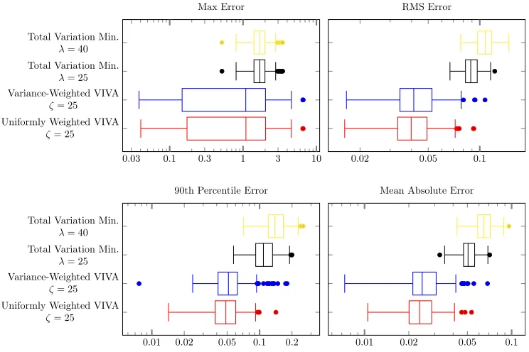
68 Performance of online estimators evaluated using piecewise linear signal (burst
LIST OF ILLUSTRATIONS xiii
69 Performance in stable regions (transition bands excluded) of online estimators evaluated using piecewise linear signal (burst noise), N = 500, analysis of value
estimate 72
70 Performance of online estimators evaluated using piecewise linear signal (burst
noise), N = 500, analysis of rate estimate 73
71 Performance in stable regions (transition bands excluded) of online estimators evaluated using piecewise linear signal (burst noise), N = 500, analysis of rate
estimate 73
B.1 Fit using many conjoined piecewise-linear segments 99
E.1 Signal with “sloop” shape, with accompanying “measurement noise” 108
E.2 Noiseless signal with “sloop” shape and minimum-MSE polyline approximations by
segment count 109
E.3 Comparison of computational complexity of residual minimization using fixed segment count and bicriterion regularization with and without pruning, signal is the
noiseless “sloop” shown in Figure E.1 110
E.4 Comparison of computational complexity of bicriterion regularization via pruned dynamic programming, with and without truncation heuristics, applied to the
noiseless “sloop” shown in Figure E.1 110
E.5 Minimum-MSE polyline approximations for “sloop with measurement noise” signal 111
E.6 Comparison of computational complexity of residual minimization using fixed segment count and bicriterion regularization with and without pruning, signal is the
“sloop with measurement noise” shown in Figure E.1 112
E.7 Comparison of computational complexity of bicriterion regularization via pruned dynamic programming, with and without truncation heuristics, applied to the
“sloop with measurement noise” shown in Figure E.1 112
E.8 Signal with “gaff cutter” shape, with accompanying “measurement noise” 113
E.9 Noiseless signal with “gaff cutter” shape and minimum-MSE polyline approximations
for several segment counts 114
E.10 Comparison of computational complexity of residual minimization using fixed segment count and bicriterion regularization with and without pruning, signal is the
noiseless “gaff cutter” shown in E.8 115
E.11 Comparison of computational complexity of bicriterion regularization via pruned dynamic programming, with and without truncation heuristics, applied to the
noiseless “gaff cutter” shown in Figure E.8 115
E.12 Optimal polyline approximations for “gaff cutter” signal with added noise and with
fixed segment count 116
E.13 Comparison of computational complexity of residual minimization using fixed segment count and bicriterion regularization with and without pruning, signal is the
“gaff cutter with measurement noise” shown in E.8 117
E.14 Comparison of computational complexity of bicriterion regularization via pruned dynamic programming, with and without truncation heuristics, applied to the “gaff
1
CHAPTER 1
Background
This chapter describes the medical scenario that motivated development of a novel online denoising algorithm. Shock, defined as “a life-threatening, generalized maldistribution of blood flow resulting in failure to deliver and/or utilize adequate amounts of oxygen” (Antonelli et al., 2007) occurs acutely in victims of trauma, infection, and burn. Resuscitation of shock requires individualized care that accounts for patient-specific responses, as responses that differ from the “textbook case” are prevalent. Computers can assist with provision of fluid and drug therapies used to resuscitate shock, as well as decision support and alarming. However, hemodynamic optimization requires accurate and timely measures of both therapy delivered and patient re-sponse. The harried environments in which medicine is practiced make obtaining these signals quite challenging. Existing methods of noise removal are poorly suited to the task.
1.1.
The Value of Infusion Monitoring
1.1.1. Shock is a Major Factor in Preventable Deaths. Traumatic injuries cause more deaths of patients aged 40 and under than any other cause (Spinella and Holcomb, 2009), causing approx-imately 90,000 deaths annually in the USA alone. Of these, Spinella and Holcomb estimate that 10,000 or more result from inadequate treatment of hemorrhagic shock resulting from survivable injuries. Amongst battlefield injuries, the prevalence of traumatic hemorrhage is even higher, with one fifth of fatalities occurring following injuries classified as potentially survivable, due to exsanguination before reaching a medical treatment facility (Eastridge et al., 2012). According to Newgard et al. (2010), receiving care from an experienced trauma team at a major trauma center is crucially important to outcome, while time spent pre-hospital and in transport is not, but this considered only transport times up to two hours and assumes that adequate resources are available to keep the casualty stable, something that often is not true on the battlefield.
The US military has proposed to address this need by (1) using electronics to bring exper-tise to combat medics (2) evacuate casualties to definitive care earlier (3) improve care during transport . Several key initiatives include use of unpiloted drones, having delivered supplies to forward troops, to perform timely medical evacuation through environments too dangerous to hazard human care providers (ONR BAA 12-004 CONOPs). An autonomous critical care system (ACCS) is under development by the Office of Naval Research. The ACCS will provide decision support to a corpsman in the field to help stabilize and prepare a patient for transport, then manage a patient during medical evacuations, either autonomously or with the help of remote guidance from telemedicine caregivers (ONR BAA 11-012). The ACCS can also be used in med-ical facilities as a force multiplier by aiding in hemodynamic management, thus requiring less medical provider time per patient.
Shock resulting from severe sepsis has a mortality rate from 28 % to 50 % (Wood and Angus, 2004), killing over 100,000 hospital patients annually (Martin et al., 2003). Burn patients also are at risk of hypotensive shock, either from fluid loss induced by the burn, or resulting from secondary infections.
1.1. THE VALUE OF INFUSION MONITORING 2
1.1.2. Shock is Treated by Optimum Fluid Therapy. Infusion of fluid to increase circulating blood volume (Sanford and Herndon, 2001) is essential to resuscitation of shock victims because it sequentially increases venous return, cardiac stroke volume, and volumetric flow rate (“car-diac output”) (Gagnon, 2009; Antonelli et al., 2007; Kramer et al., 2007a). Increased car(“car-diac output will, ceteris paribus, both increase the net oxygen delivered to tissues and increase tissue perfusion. However, fluid infusion is a two-edged sword, as fluid overload also puts the patient at risk (Perel, 2008; Spinella and Holcomb, 2009). Increased vascular pressure increases effluent flow rates, making it more difficult for clots to form (coagulation), and also increases strain on newly formed clots, which may cause them to fail and internal bleeding to resume (Spinella and Holcomb, 2009). Dilution of blood with infusate also reduces the concentration of oxygen carriers and clotting factors (Spinella and Holcomb, 2009).
Additional effects are related to characteristics of the particular fluid used (Guha et al., 1996; Kramer et al., 2007a). Use of saline solutions causes a decrease in protein concentrations, reduced colloid osmotic pressure, and increased leakage of water into the surrounding tissues (Saffle, 2007; Kramer et al., 2007a), causing swelling (“edema”), while solutions of hypertonic saline or colloids have the opposite effect Guha et al. (1996); Fodor et al. (2006). If this occurs in the lungs (“pulmonary edema”), the increased aveolar wall thickness will reduce the effectiveness of gas exchange (Holm et al., 2004), and may result in lower arterial oxygen saturation. If swelling occurs inside the abdomen, pressure may be exerted on vital abdominal organs, causing collapse of veins and impeding blood flow and organ function. This condition is known as “intra-abdominal hypertension” and if unchecked leads to organ failure designated “abdominal compartment syndrome” (Saggi et al., 2001; Pham et al., 2008; Salinas et al., 2008; Cancio, 2014). Edema also increases the risk that a burn injury will become septic (Hoskins et al., 2006; Salinas et al., 2008); conversely sepsis increases edema (van der Heijden et al., 2009). If the infusate is not warmed to body temperature, it can contribute to hypothermia, negatively affecting coagulation that may already be compromised by acidosis (Tsuei and Kearney, 2004).
For all these reasons it is desirable to infuse the minimal volume needed to achieve clinical goals (Cancio, 2014). Yet providers continue to infuse burn patients with significantly more fluid (Kramer et al., 2007b; Salinas et al., 2008; Oda et al., 2006) than called for by consensus rec-ommendations (Pham et al., 2008), and these large fluid volumes are implicated in development of abdominal compartment syndrome (ACS) (Oda et al., 2006; Saffle, 2007). Resuscitation fluid is associated with ACS in non-burn patients as well (Balogh, 2003; Sugrue, 2005). According to Sugrue (2005), 5 % of intensive care patients suffer from ACS. Mortality varies between 25 % and 75 % (Balogh et al., 2003).
1.1.3. Goal-Directed Therapy Achieves Better Outcomes. One possible explanation for the persistence of burn care providers in choosing to err on the side of extra fluid is that under-resuscitation represents acute risk, while harm resulting from over-under-resuscitation manifests multi-ple hours if not days in the future. Often the providers are convinced that fluid volumes exceeding the formulaic calculations are truly needed in these patients. Yet evidence shows that when fluid is systematically managed using objective goal-directed rules, fluid volumes are generally less than predicted by the Parkland formula without leading to under-resuscitation (Salinas et al., 2011; Oda et al., 2006; Arlati et al., 2007), and in fact achieve better outcomes (Salinas et al., 2008).
The advantages of goal-directed (explicit feedback loop) therapy are not limited to burn patients either. Outcomes in sepsis patients improved following implementation of goal-directed therapy (Otero, 2006; Perel, 2008). A meta-analysis performed by Hamilton et al. (2011) found significant improved outcomes in a broad range of high risk surgical and critical care patients.
1.1. THE VALUE OF INFUSION MONITORING 3
Fortunately, both knowledge-based treatment and feedback control are amenable to computer automation.
1.1.4. Research Demonstrates that Decision Support and Closed-Loop Control of Hemody-namics is Possible. In fact, there have already been successes in implementation of closed-loop management of fluid (Rafie et al., 2004; Ying et al., 2002; Hoskins et al., 2006; Salinas et al., 2008; Kramer et al., 2008; Vaid et al., 2006; Rinehart et al., 2011, 2012; Meador, 2014; Cancio, 2014), vasodilators for relief of hypertension (Hammond et al., 1979; Ying et al., 1992), and vasoconstrictors for correction of normovolemic hypotension (Yu et al., 1992; Rao et al., 1999, 2003; Ngan Kee et al., 2008) in large mammals and human patients. Automatic sedation has been demonstrated as well (Bibian et al., 2005; Hemmerling, 2009; Struys et al., 2001). These closed-loop control studies have been performed during a variety of surgical and intensive care scenarios as well as first responder / point of injury simulations. Even though the computer does not have knowledge of upcoming surgical actions and consequences, the responsiveness of silicon processors results in making decisions about new data more quickly; reaching targets faster, with less overshoot; and managing endpoint variables more precisely than can a human provider with multiple responsibilities.
1.1.5. Limitations of Automated Fluid Delivery using a Fixed Control Law. While the suc-cessful closed-loop tests demonstrate the potential rewards of using computers to automatically manage hemodynamics, these studies are limited in scope and it would be premature to believe that the algorithms are ready for broad deployment. In particular, the research animals were healthy apart from the intentionally inflicted injury and patients were selected using criteria that excluded complications. While these restrictions are perfectly understandable considering the research goals of reproducibility and cohort comparison, and the ethical goal of patient safety, they do not address questions about safety and efficacy on a broader population. Inter-patient variability that was largely excluded by study criteria may lead to poor outcomes. For example, controlling fluid infusion to sepsis patients based on a target of central venous pressure may cause overinfusion (Perel, 2008). According to Preisman (2005), single-variable optimization of cardiac output may lead to fluid overload; as many as 50 % of patients may be unresponsive (in the sense of increasing stroke volume) to fluid.
In extreme cases, the negative effects of fluid infusion could adversely affect the feedback variable, setting up a positive feedback loop that demands fluid therapy more insistently even as it drives the patient ever further from the target. In their work on closed-loop sedation, Bibian et al. (2005, 2004); Zikov and Bibian (2014) explain the importance of bounding the uncertainty of patient response and defining the controller’s region of convergence and stability. A key insight comes from Haddad and Bailey (2009), “[...] it has been assumed that stability follows from the pharmacokinetic/pharmacodynamic model. However, this is not the case since these controllers do not account for full model uncertainty, unmodeled dynamics, exogenous disturbances, and system nonlinearities.”
1.1.6. Controllers Benefit from Automated Response Analysis. Individualization of models through observing output response for the purpose of per-patient parameter identification, even if only a subset of parameters can be determined (partial parameter identification), can be used to improve controller performance (Bibian et al., 2004). Some control techniques, such as model adaptive control, explicitly use the subject-specific parameter values. Other controllers may be able to account for reduced uncertainty by gain adjustment.
1.2. PRACTICAL MEASUREMENT OF INFUSION RATE 4
1.1.7. “Electronic Doctor” Diagnosis and Prescription will Rely on Automated Response Analysis. Like the human decision process (Kahneman, 2011), autonomous critical care systems of the future will consist of a slow “reasoning” expert system performing diagnosis and selection of therapies and drugs, with fast “reacting” closed-loop controllers carrying out these therapies. Several closed-loop controllers have already been mentioned. Gholami et al. (2012) states that
It is important to note that expert systems are already in widespread use in other branches of medicine, more prominently in disease diagnosis, where the system inputs are the patient’s details and symptoms, and the system outputs are probable diagnoses, recommended treatments or drugs which may be prescribed. Such systems are typically open-loop and may be regarded as rule-based search engines to help the clinician in his/her mapping of a given set of symptoms to a possible cause (disease).
and furthermore provides a framework for application of Bayesian expert systems in the fast closed-loop portion of the system. This is typically seen as initial encoding of care provider knowledge heuristics, which are later replaced by robust and adaptive controllers as dynamical system models are developed.
One key element that remains is the forwarding of performance information from the reac-tion layer to the reasoning layer, which may take acreac-tions such as alarming, swapping controller implementations for one expected to yield better performance on the particular patient, or discon-tinuation of an ineffective therapy. Parameter estimation using Kalman filters has been described in Luspay and Grigoriadis (2014). This and similar adaptive techniques will provide the reasoning system with the information needed to manage inter-patient variability.
1.2.
Practical Measurement of Infusion Rate
1.2.1. Effects of Erroneous Infusion Rate. Because assessment of response to fluid bolus is intended for computer-assisted diagnosis, computerized alarming, closed-loop controllers checking preconditions that assure controllability and stability, and eventually for automated planning of patient care, the hazard of basing this assessment on invalid input data has potential to lead to harm. The assessment aggregates infusion and response data over a time interval, providing reduced sensitivity to small or transient errors in the input signal, so the input signal (infusion rate) must be known within these tolerances.
1.2.2. Need for Independent Rate Measurement. When the infusion rates of IV pumps are set by computerized control, it is tempting to accept the control signal as a perfectly accurate input signal. However, actual flow rates vary from requested rates due to variations in resistance, source pressure, and backpressure, as well as automatic safety shutdown if air or occlusion is detected. Hospital pumps controlled via front panel may or may not report the currently set rate via a computer interface. Moreover, care providers give some fluids without the aid of pumps. Manually delivered fluids are particularly common in operating rooms. Furthermore, some infusers offer relative control of flow without providing accurate flow rate information. Controllers which fail to account for actual flow rates lead to windup and improper adaptation (Haddad and Bailey, 2009). For these reasons, having an independent measure of infusion rate is helpful.
1.3. EXISTING METHODS FOR DENOISING PIECEWISE SIGNALS 5
signals. Environments with significant mechanical vibration pose particular obstacles to using load cells for infusion monitoring. Even in fixed settings, small errors in weight measurements lead to large uncertainty in rate calculations. For example, an error of only 0.1 g, if the time resolution is 10 seconds, leads to a flow rate error of 0.6 mL/min or 36 mL/h. And the problem increases with higher time resolution.
1.2.3. Infusion Monitoring System Prototype. A four channel “smart IV pole” IV bag moni-toring system to use load cells to continuously measure the weight of IV bags has been conceived in the UTMB Resuscitation Research Laboratory (Galveston, TX) and designed and built by Sparx Engineering (Manvel, TX). UTMB researchers developing smart hemodynamic resusci-tation components for the Navy ACCS have used this load cell system to record infusion data during fluid resuscitation studies of hemorrhagic and burn shock in animal models. The Texas Instruments LMP90099 analog-to-digital converter used in this system samples load cell readings 53.66 times per second with a system error of±1 g (0.2 g after averaging). The system undergoes two-point offset and gain calibration before each use. Data collected using this system consists of periods of valid readings with additive limited measurement noise, interspersed with short-duration burst noise caused by mechanical forces on either side of the load cell (IV pole or IV bag). In addition, following manipulation of the IV bag, the data are frequently observed to exhibit underdamped oscillation due to pendulum action of the IV bag.
Several different approaches may be taken to denoising the flow rate estimate. Classical lowpass filtering trades time resolution for reduced error. Regularization methods rooted in optimization theory attempt to achieve low errors and good time resolution by finding the simplest signal that is consistent with the measured data. A regularization problem was stated which encodes the domain knowledge that care providers infrequently change the infusion rate. I developed the Viterbi-Inspired Variation Assessment (VIVA) method to efficiently perform this
`0norm regularization. Further development of the VIVA method added time-varying weighting to reduce sensitivity to burst noise.
Denoising is less critical for other applications of the load cell data, such as detection of IV bag depletion or calculation of cumulative delivered fluid, which are impacted less by measurement noise. But these too benefit from identification of bag changes and rejection of burst noise from mechanical impacts on the IV pole.
1.3.
Existing Methods for Denoising Piecewise Signals
1.3.1. Bicriterion Model
In the search for the maximum-likelihood estimate{x˜k}of the underlying signal {xk}, it is natural to use a bicriterion objective function which seeks both agreement with the observations
{yk} and simplicity of description. Simplicity may be motivated by domain knowledge that control actions are few or because a short (compressed) representation is desired to simplify communication, storage, and further analysis. Then
(1.1) ˜x= argmin
x0
(x0) +ζf(x0)
where (x0) represents a goodness of fit “distance” from the observation sequence, f(x0) represents the control burden, andζis a weighting coefficient controlling a tradeoff between the two.
The usual metric for goodness of fit is integral-square residual error, which for sampled measurements becomes a discrete sum:
(1.2) (x0) =
N X
k=1
1.3. EXISTING METHODS FOR DENOISING PIECEWISE SIGNALS 6
This corresponds to negative log-likelihood in the case of additive i.i.d. Gaussian noise (AWGN). In the case of non-stationary noise, a weighting function may be included:
(1.3) (x0) =
N X
k=1
ck(x0k−yk) 2
For control actions which act on either value or rate of observations, the control burden may be expressed as the number (cardinality) of non-zero control inputs
(1.4) f(x0) = card (∆px0)
wherepexpresses the controller-observer relationship, with particular interest in the values
(1.5) p∈
2 rate control
1 value control
This problem is relevant to many areas of operations research, with related work appearing in the changepoint, linear programming, integer programming, dynamic programming, and convex optimization literature. Existing work falls into several classifications:
• In-exact solutions, typified by greedy algorithms
• Convex relaxations
• Exact solutions with poor scaling
• Dynamic programming
1.3.2. Inexact Methods
1.3.2.1. “Greedy” Step-Fitting Algorithms. Another active research area in biology which requires denoising piecewise-constant data is the study of protein regulation of microtubule as-sembly (Kerssemakers et al., 2006). In 2008, Carter et al. used artificial data sets analogous to kinesin motion to compare four methods for automatic resolution of individual steps, concluding that the best of these was the chi-squared minimization method developed by Kerssemakers et al. (2006). This method uses a fractal-like procedure whereby the entire dataset is split into two at the point which minimizes residual chi-square measure. The procedure is then repeated on each segment found, and the new step which reduces residual chi-square the most is accepted. The algorithm also provides a quality measure which terminates the iteration. In the developers’ own words, “Once found, the step-locations do not change anymore, although the associated step sizes continue to change as they depend on the location of the neighboring steps” making this a greedy algorithm. This approach is similar to the Binary Segmentation method described in the changepoint literature (Killick et al., 2012), but the Kerssemakers et al. method incorporates an additional termination condition designed to prevent overfitting.
1.3.3. Convex Methods
1.3. EXISTING METHODS FOR DENOISING PIECEWISE SIGNALS 7
0 2 4 6 8 10
−10 −5 0 5 10
Sample Number (thousands)
Measured Original Signal
TVMλ= 80
Figure 1. In Total Variation Minimization, the penalty function biases the estimate for extreme segments
0 2 4 6 8 10
−10 −5 0 5 10
Sample Number (thousands)
Measured Original Signal
TVMλ= 80
1.3. EXISTING METHODS FOR DENOISING PIECEWISE SIGNALS 8
2000 2001 2002 2003 2004 2005 2006 2007
6.6 6.7 6.8 6.9 7 7.1 7.2 7.3
Year log price
Source Data VIVA, High Sparsity VIVA, Tight Fit
`1Trend Filtering (Kim 2009)
Figure 3. `1Trend Filter is systematically biased toward shallow changes in slope
Table 1. Comparison of residual error and sparsity of trend-filter estimates
Method RMS residual Segmentation
# Changepoints Slope Threshold
`1 Trend Filtering 0.0314 12 10−4
(Kim et al., 2009) 42 10−6
VIVA (Tight Fit) 0.0283 9 10−10
VIVA (Sparse) 0.0319 6 10−10
1.3.3.2. Trend Filtering. Kim et al. demonstrated use of global`1 bicriterion regularization for fitting polyline models. These models are used extensively in a variety of financial and biological applications (Kim et al., 2009). Considering the stock price curve fitting problem which appeared as Figure 2 in Kim et al. (2009), comparison of the`1trend filtering result to two other piecewise-linear curves shows that this relaxation exhibits the same systematic sub-optimality as total variation minimization, manifesting as underestimation of changes in slope and failure to obtain a truly sparse description (Figure 3, Table 1).
1.3.3.3. Other Interior Point Methods. Julian et al. (1998) performs fitting of piecewise-affine multidimensional surfaces to sample data by proposing partition boundaries and performing descent using a Newton-Gauss algorithm to exponentially converge to a local minimum. When the conditions for global optimality are not met, the algorithm attempts to escape local minima by restarting the algorithm from new initial partitions. Problems with larger numbers of hyperplanes are addressed by optimizing using a smaller number to obtain an initial partitioning for the larger problem. This method is avoided for data with large numbers of segments due to its poor scaling with facet count.
Xu et al. (2011) fits images with a reduced variation cardinality using an iterative algorithm that alternates between identifying edges and then smoothing between them. Their method performs simultaneous optimization across the entire dataset and works only for the piecewise-constant case. Since less expensive methods exist for finding exact solutions in the one dimen-sional case, no attempt will be made to adapt it for real-time use.
1.3.3.4. Advantages of`0 Regularization. It is interesting that, aside from its convexity, the most valuable attribute of`1 norm regularization is that it approximates finding solutions to the
1.3. EXISTING METHODS FOR DENOISING PIECEWISE SIGNALS 9
tA ti tB
−10
−5 0 5 10 15
Measurement
bi= 0 bi= 1
Figure 4. The binary sequencebj segments the measurement sequenceyj into independent constant segments
problem will not be convex, and is described in the literature as intractable.” Undissuaded, Chartrand then goes on to show that using descent methods with this non-convex `p norm is statistically likely to find a solution with the globally optimal sparsity pattern, and that even local minima generate better reconstructions of sparsely sampled signals than found using the`1 norm. Furthermore Xu et al. (2011) constructs signals for which the`1 norm heuristic fails to find the optimal sparse solution.
1.3.4. Equivalent Mixed-Integer Models
Another expression of the maximum likelihood estimation problem is as a mixed-integer quadratic program (Roll et al., 2004). Augment the problem with additional binary variables, which segment the measurement sequence (Figure 4):
(1.6) bk =
(
1 ∃i,(k−1)Tv<Ti−t1≤kTv
0 otherwise
whereTv is the time resolution with which it is desired to locate step changes.
The complete MIQP model for piecewise-constant estimation with the `0 norm (variation cardinality minimization) objective function is:
(1.7)
minimize (x0−y)T(x0−y) +ζ1Tb0
subject to −x0k +xk+10 −M b0k ≤ 0 ∀k x0k −x0k+1 −M b0k ≤ 0 ∀k b0k∈ {0,1} ∀k
1.3. EXISTING METHODS FOR DENOISING PIECEWISE SIGNALS 10
(1.8)
minimize (x0−y)T(x0−y) +ζ1Tb0
subject to (ti−ti+1)x0k−1 + (ti+1−ti−1)x0k + (ti−1−ti)x0k+1 −M b0k ≤ 0 ∀k (ti+1−ti)x0k−1 + (ti−1−ti+1)x0k + (ti−ti−1)x0k+1 −M b0k ≤ 0 ∀k
b0k∈ {0,1} ∀k
So too is this piecewise-linear estimation problem with the continuity constraints removed (periodic sampling assumed for simplicity of notation):
(1.9)
minimize (x0−y)T(x0−y) +ζ1Tb0
subject to −x0k−1 + 2x0k −xk+10 −M b0k−1 −M b0k ≤ 0 ∀k x0k−1 −2x0k +x0k+1 −M b0k−1 −M b0k ≤ 0 ∀k b0k∈ {0,1} ∀k
Although it is easier to solve exactly, the model is more complex.
In contrast, the`1 norm (total variation minimization) formulation is (piecewise-constant, mutatis mutandis for piecewise-linear with continuity):
(1.10)
minimize (x0−y)T(x0−y) +ζ1Td0
subject to −x0k +xk+10 −d0k ≤ 0 ∀k x0k −x0k+1 −d0k ≤ 0 ∀k
which is a quadratic program (with linear constraints).
If instead of minimizing the integral-square residual error, the integral absolute residual error (`1 norm) is minimized,
(1.11) (x0) =
N X
k=1
|x0k−yk|
then the objective function becomes linear, forming a mixed-integer linear program (MILP):
(1.12)
minimize 1Tr0+ζ1Tb0
subject to −x0k +xk+10 −M b0k ≤ 0 ∀k
x0k −x0k+1 −M b0k ≤ 0 ∀k
−x0k +yk0 −rk0 ≤ 0 ∀k x0k −yk0 −rk0 ≤ 0 ∀k b0k∈ {0,1} ∀k
Naturally it is also possible to use the `1 norm for both goodness of fit and simplicity of description, in which case a linear program is obtained. Another related linear program is obtained from the minimax residual:
(1.13) (x0) =X
i
max
Ti≤kTv≤Ti+1
|x0k−yk|
1.3.5. Methods of Solving Integer Programs
1.3. EXISTING METHODS FOR DENOISING PIECEWISE SIGNALS 11
1.3.5.1. Symmetry reduction. Symmetry (when mapping between descriptive parameters and solution is not injective, for example when permutations of the parameters are equally valid) poses a particular problem for branch-and-bound, since even the optimal cost is not strong enough to prune subproblems that contain another optimum (Barnhart et al., 1998).
The binary variables are paired with observations in the MIQP models given, so if the obser-vation times are distinct, there is no symmetry. In case of multiple obserobser-vations at a single time, this could become problematic. Especially when there is no continuity constraint, if observations occur simultaneously with a jump discontinuity (to within measurement time precision), the wrong partition of observed values could lead to suboptimality. However rather than introducing symmetry, one need only consider two orderings, corresponding to either ascending or descending sort of the observations.
A similar approach is used by Roll et al. (2004) to address estimation of a monotonic piecewise-affine function (jump discontinuities allowed, provided they are in the direction pre-serving monotonicity) pre-serving as the non-linear output mapping of a Wiener model. Roll et al., not having knowledge of the abscissa, breaks symmetry by sorting observations by the ordinate, resulting in computational complexity which is combinatorial – polynomial in the length of the input data, but exponential in the number of changepoints. This ordering could prove problem-atic if the effect of noise swaps two (or more) observations which lie either side of a changepoint. Due to this concern and the high complexity, this approach would not be used for the simpler case of finding piecewise functions of time.
1.3.5.2. Bound strengthening methods. Because branching increases complexity exponen-tially, effort is often expended on further constraining the linear / convex relaxation to produce a feasible solution. Branch-and-cut and branch-and-price (Barnhart et al., 1998) are complemen-tary methods that tighten the bounds of the relaxed problem. Gomory cuts specifically tighten subproblems by adding bounds on a variable whose integrality is violated by the relaxed opti-mum. For MILP problems (linear objective function), various cutting planes including Gomory cuts, lifted-cover inequalities, flow cover inequalities, and gub-cover inequalities can be automat-ically added by such solvers as bc-opt (Cordier et al., 1999), MPSARX, MINTO, and MIPO. While not directly applicable to the MIQP models, it is likely that commercial solvers such as CPLEX (IBM) and would be able to apply cuts to reduce the required branching.
Branch-and-price aids in the optimization of problems with many variables (as these MIQP models have) by optimizing using a small basis set. Other integer variables are exchanged with the basis set (“priced in”) depending on the residual cost associated with them.
Branch-and-reduce Ryoo and Sahinidis (1996), implemented in the BARON solver (Sahinidis, 1996) also performs automated bounds tightening.
Although these methods lead to more efficient solution than exhaustive brute-force search, they do not take full advantage of the problem structure and require solving numerous subprob-lems each of similar complexity to the best dynamic programming approaches. They remain useful approaches for MILP and MIQP such as the hinging hyperplane fitting algorithm of Roll et al. (2004) and Toriello and Vielma (2012)’s models for grid tesselation using triangles and surface fitting using convex piecewise-affine functions.
1.3. EXISTING METHODS FOR DENOISING PIECEWISE SIGNALS 12
1.3.6. Related Work in Dynamic Programming
1.3.6.1. Curve Estimation in the Dynamic Programming Literature. Dynamic programming found applications to piecewise curve estimation quite early. Bellman (1961) described a simple approach to finding the sequence of N disjoint segments that most closely approximated, in a minimum integral-square residual error sense, an integrable function over a fixed interval. For this method the abscissa of each end-point is constrained to a discretization of the interval. The state space was defined by the coordinate pair (right edge of interval, number of segments used). The computational complexity therefore is O(u2NN) comparisons, where uN is the number of discrete steps quantizing the interval. If memoization is used,uN coefficient-search steps may be performed inO(uN) time.
Continuity between segments was considered in Bellman and Roth (1969), where a polyline of
N (joined) segments is used to approximate an arbitrary continuous curve, where all join points are required to lie on lattice points (both abscissa and ordinate are quantized). The state space is the triple (abscissa of end point, ordinate of end point, number of segments used) leading to a complexity ofO(h2v2N) comparisons, where ordinate and abscissa are quantized intov andh discrete steps, respectively. Bellman and Roth uses a somewhat unusual cost function, the sum of per-segment maximum absolute error.
Both these algorithms exhibit poor scaling, but motivated further use of dynamic program-ming.
Another pioneer in use of curve fitting via dynamic programming was Guthery (1974), whose notation ofk for the number of partitions andn for the number of data samples, shall be used going forward due to its clarity. He first offers the insight that, given sufficient space, memoization reduces the number of coefficient-search steps in the disjoint piecewise estimation problem to
O(n2) fromO(n2k) (and the number of residual calculations in the piecewise-continuous problem is likewise reduced by a factor of k), although the number of comparisons remains linear inN. Then Guthery introduces Partition Regression, which estimates models for sampled data using piecewise parameterized curves. The first-order auto-regressive models used for curve segments permit dynamics which are exponential in time and non-linear in the coefficients. The method is unsuitable for high sample rate data, not because of scaling complexity, which is quadratic in number of samples, but because the pairwise treatment of data amplifies high frequency noise. Use of higher order auto-regression models is clearly possible but the modeling of individual segments might then become expensive. Recognizing that combining the individual partition models into a single continuous curve might be sub-optimal, Guthery recommends adopting the selected partition boundaries and performing concurrent reoptimization of the parameters.
1.3.6.2. Reception of Digital Codes. Maximum likelihood recovery of signals from noisy mea-surements using log-likelihood as the goodness-of-fit metric and exploration of a tree dates to Fano’s sequential decoder. In the sequential decoder (Fano, 1963), which is applicable to digital signals which are members of a discrete set of levels and with a known symbol duration, the n-ary tree representing the signals is explored depth-first, with one one branch fully expanded, and backtracking is used to trigger exploration of other branches based on a mutual information heuristic. The backtracking distance is bounded either by finite memory in the decoder, or the desire to make a decision after a finite delay.
1.3. EXISTING METHODS FOR DENOISING PIECEWISE SIGNALS 13
path for that state. (Highest likelihood corresponds to dominance unless the noise properties of the channel are correlated in ways that Viterbi termed “pathological”) Because the number of survivor paths is limited by the number of encoder states, the storage requirements do not depend on signal length, and decoding computational requirements are linear in signal length.
Although they did not use the term “memoization”, the technique was applied by both Fano and Viterbi, who noted that the log-likelihood of independent symbols shared terms between multiple paths, and computed metrics using the partial sums and new samples. And Viterbi’s survivor-selection is, in all but name, Bellman’s “Principle of Optimality”.
In these decoders the timing is assumed to be known. More likely is the case when the time between steps is known but the time of the first bit is not, in which case clock recovery is employed to determine the phase, and the decoding results are processed by a synchronizer to find which symbol is the first in a message. Clock recovery circuits may themselves employ maximum likelihood techniques (Kobayashi, 1971).
1.3.6.3. Pruned dynamic programming. While the state enumeration methods used by the Viterbi decoder and subsolution enumeration for curve fitting on a lattice (Bellman and Roth, 1969) are powerful for guaranteeing optimality, they require imposing coarse quantization on the signal to restrict the number of potential states.
The approximation method used by Bellman (1961) and later given the name “Segment Neighborhood” eliminates quantization error by changing the ordinate from part of the sub-solution identifier to an attribute of the sub-solution. The subsub-solutions are instead identified by the number of input data points included and the number of segments used. Computation re-quiresO(kn2) cost evaluations. For analysis in order of data arrival, the storage requirement is for O(kn) subsolutions identified by sample index and number of segments. For retrospective analysis when the iteration order can be reversed, onlyO(n) subsolutions need to be stored.
Rigaill (2010) improves this situation considerably, by making the abscissa part an attribute as well, and identifying subsolutions by number of segments used and set of ordinate intervals over which the particular subsolution is optimal. When the optimal set for any prior subsolution becomes empty, that subsolution is dropped from consideration. In this “Pruned Dynamic Pro-gramming” algorithm, the total number of intervals which must be tracked is observed to remain relatively constant in many realistic datasets, although degenerate cases such as monotonically increasing measurements yield no pruning and once again lead toO(kn) growth in the number of stored subsolutions. Rigaill completely commits to in-order data processing and notes that this permits real-time applications, although no evaluation of online estimation error performance is conducted.
Meanwhile, Yao (1984) showed that when the likelihood of a change in any single sample interval is time-invariant (leading to geometrically distributed segment durations) and the rela-tionship between its probability and the probability distribution of noise is known, then recursion and induction may be applied (reinventing dynamic programming) to find the maximum likeli-hood signal estimate in O(n2) steps and O(n) storage, with no dependence on the number of segments. This method was later given the name “Optimal Partitioning”.
1.4. REAL-TIME IMPLICATIONS 14
1.4.
Real-Time Implications
The greedy chi-squared minimization and total variation minimization algorithms have excel-lent time complexity. However, both require the entire data set to be available; the final iteration of residual chi-squared minimization can introduce a step anywhere in the entire dataset, while each iteration of total variation minimization updates the entire estimate vector. Therefore, to use these algorithms in near real-time requires running the entire O(n) algorithm at each of
O(n) data points. Note that convergence speed of total variation minimization is improved by using the prior result as an initial value, but this only lowers the constant factor – running the algorithm online still has quadratic overall complexity.
Integer Programming methods would be extremely expensive to repeat on an ever-expanding dataset. The optimal solution to the prefix data would lead directly to a known feasible solution and bound on the optimal cost; however due to the weakness of the relaxation, a large search space would still need to be explored.
The previously discussed dynamic programming methods are capable of processing data in-order, so running them online during measurement is efficient. However the Rigaill (2010) pruned DP method requires that the number of segments be bounded a-priori. Allowing both incoming data and growth in the number of segments would be prohibitive in storage complexity. Yet not knowing how many segments to reserve for fitting future changepoints precludes producing estimates in real-time with a fixed bound on segment count, since which of the currently-optimal (for different segment counts) solutions to use cannot be determined.
Killick et al. (2012)’s PELT method lends itself very well to in-order evaluation on causal datasets. Indeed, the simplest form of the VIVA algorithm, although independently developed using a different proof, is an instantiation of PELT. However PELT is inapplicable to connected piecewise-linear estimation and also lacks some refinements that will be shown to reduce online estimation error.