Simple concepts in computational mechanics – do they really work? Milos Kojic
Belgrade Metropolitan University - Bioengineering Research and Development Center BioIRC Kragujevac, Prvoslava Stojanovica 6, 3400 Kragujevac, Serbia
Houston Methodist Research Institute, The Department of Nanomedicine, 6670 Bertner Ave., R7-117, Houston, TX 77030
Abstract
The aim of this paper is to present some of simple concepts introduced by the author. The author has found, after decades of work in computational mechanics, that it is (almost always) true that the simpler concept – the more robust and attractive methodology is. For the sake of completeness a small review of the fundamental relations and their counterparts in Finite Element (FE) framework are presented. The topics span from solid and fluid mechanics to biomechanics, field problems and multiscale diffusion. Typical examples illustrate the application of the simple concepts. Altogether, a goal of this article might be a motivation for solving more complex problems in a simple manner.
Keywords: Finite Element Method, solid-fluid interaction, stress integration, multiscale diffusion, microstructural flow, incompressible deformations of solid
1. Introduction
In this section we present the fundamental laws and equations, followed by the corresponding FE balance equations, where the simple concepts are introduced.
2
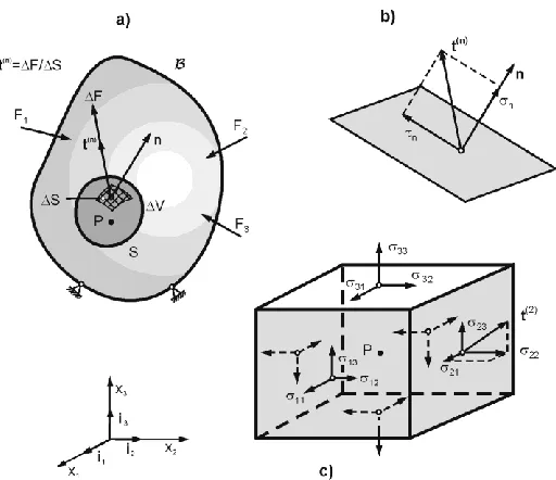
Fig. 1 Definition of stresses in continuum mechanics (M. Kojic et al. 2008).
0, , 1, 2,3
V ik
i i
k
u f i j
x
(1)
where ikare stresses, is material density, ui are components of acceleration and V i
f are volumetric force components; summation of the repeated index k (k=1,2,3) is implied. The FE incremental-iterative balance equation of a finite element is
( )i ext intL NL
K K U F F (2)
where KL and KNL are (geometrically) linear and nonlinear stiffness matrices, ( )i
U are increments of nodal displacements at iteration “i”, and ext
F and Fint are external and internal nodal forces. The matrices and nodal vectors correspond to the values at the previous iteration, but we omit this indication for simplicity of writing. Detailed expressions for the matrices are given elsewhere (M. Kojic et al. 2008), (K. J. Bathe et al. 1996), but we here give those used in further presentation:
T
L L L
V
dV
K B CB (3)
int T
L V
dV
F B σ (4)
where BL is the matrix relating the strains and displacements, σ is the stress tensor, V is element volume, and the constitutive matrix C represents the relations between stresses i and
strains ej (in one-index notation),
i ij
j
C e
This matrix is defined by two material constants, but in case of complex material behavior, it can depend on the current strains as well as on the history of material deformation. Evaluation of this matrix and stresses in terms of the current state of deformation is a challenging task and some simple solutions are given below. The above balance equation is according to the Lagrangian formulation.
In case of fluid flow, an Eulerian description of the Newton Law is commonly used so that the balance equations (1) are slightly different and are called the Navier-Stokes equations,
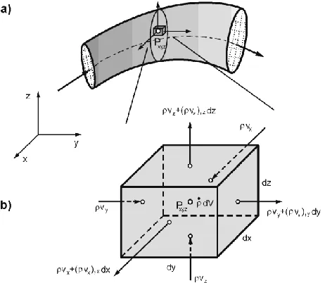
Fig. 2. Reference volume (RV) around a spatial point P in the fluid domain (a), and velocities at the RV faces (b) (M. Kojic et al. 2008).
1, 2,3; sum on : 1, 2,3
V
i i ik
k i
k i k
v v p
v f i k k
t x x x
(6)
where is fluid density (assumption is that fluid is incompressible), vi are velocities, ik are
viscous stresses, and p is pressure. Here, the stress is decomposed into viscous terms and pressure,
ik ik p ik
(7)
where ik is the Kronecker delta-symbol. The viscous stresses have a deviatoric character since the fluid is incompressible. We will emphasize in the stress integration for solids that the decomposition of stresses (7) is very important. The constitutive relations for viscous stresses are
, ,
2
ij eij vi j vj i
(8)
where is fluid viscosity, eij are the strain rates and „comma‟ means ,i / xi. The
continuity equation must be satisfied, which for incompressible fluid has a form
1 1 2 2 3 3
/ / / / 0
i i
v x v x v x v x
4
The finite element equations, which include both (6) and (9), can be written as
( )
( )
1
1
1
0
0
0
0
i ext
vv vp vv vp
i
T T
vp vp
t
t
t
M
K
K
V
F
M K
K
V
MV
P
P
K
K
(10)
where the expressions for the element matrices and vectors can be found elsewhere (M. Kojic et al. 2008; N. Filipovic 2011); V and P are nodal velocities and pressures. In case of linear elements, used further, the pressure is assumed to be uniform within the element and becomes a scalar P in the above equation.
In case of solid-fluid interaction and strong coupling approach, the system of balance equations includes both solid and fluid parts, with the common nodes and degrees of freedom at the interface. Then, the complete system consists of equations (10) and (2); eq. (2) can be written in terms of velocities as:
( ) int
1
i extt
t
M
K
U
F
F
(11)The fundamental equation for field problems, considered here for mass transfer, have a form
0
V ii i
s
k
q
t
x
x
(12)where is a field variable (concentration c in case of diffusion, potential in case of underground water flow through a porous medium – a Darcy flow ), s is a time related coefficient (equal to 1 in case of diffusion, storage in case of Darcy flow), ki are the transport
coefficients (diffusion or permeability coefficients), qV is a source term. The balance FE equations can be written as (M. Kojic et al. 2008):
( )
1 i ext 1 t
t t
M K Φ Q KΦ M Φ Φ (13)
where Φ is the nodal vector and tΦ corresponds to the start of time step; ext
Q is the external nodal flux; details about matrices are given in (M. Kojic et al. 2008). The matrix which is of particular interest in this article is the transport matrix K,
, ,
IJ j I j J j
V
K
k N N dV sum on j: j=1,2,3 (14)In case of mass transport within the fluid domain with fluid flow, equation (13) can be written as
v
ext
MΦ K K Φ Q (15)
where the convective matrix Kv is
,v
i K i
i KJ V
v N N dV
K no sum on i (16)
2. Solid mechanics
2.1. Stress integration for nonlinear material models
Constitutive material characteristics can nonlinearly depend on strains or can nonlinearly depend on other deformation dependent parameters. Then, incremental FE analysis must be performed, and the solution accuracy depends on the proper evaluation of stresses used in calculation of nodal forces (4). On the other hand, rate of convergence within iterative scheme (2) strongly depends on the calculation of the constitutive matrix (6). We first give example of metal plasticity to demonstrate how a simple concept provides general solutions.
The first important step is to realize that plastic deformation is incompressible, hence the mean stress has no effect on this part of the material deformation. Normally, we decompose the stress into deviatoric stresses Si and the mean stress m
1 33
/ 3 (written in theone-index notation)
, 1, 2,3; , 4,5,6
i Si m i i Si i
(17)
where the first three components correspond to normal and the last three to shear character.
The next crucial step is to employ the homogenous shape of deviatoric stress – elastic deviatoric strain (e'Ei ) relationships:
2 'E 2 ' P 2 ' t P P
i i i i i i i
S Ge G e e G e e e (18)
where G is elastic shear modulus, 'ei are the total deviatoric strains (e'i ei (e1 e2 e3) / 3), t P
i
e are plastic strains at start of time step, and P i
e
are increments of plastic strains. We next use the constitutive law (normality principle) for plastic strain increments:
P
i i
e S
(19)
where is a positive scalar. Taking scalar products of each the left and right-hand sides of this equation, we obtain that
3 2 P e
(20)
where eP is increment of the effective plastic strain and is the effective stress. Substituting (19) into (18), and with a use of (20), we can solve for deviatoric stresses,
*
1 3 /
t E
i
i P
S S
G e
(21)
where Si*E is the deviatoric stress corresponding to zero-increment of plastic strain (trial elastic
deviatoric stress). Taking the scalar product of the left and tight-hand sides we finally obtain a scalar equation,
*3 0
p E p
f e G e (22)
Besides this scalar equation, the yield condition at the end of time step must be satisfied,
(t p p) 0
y y
6
where (t p p)
y e e
is the uniaxial yield stress, and the equation (22) can be written as
*3 0
P E p
y
f e G e (24)
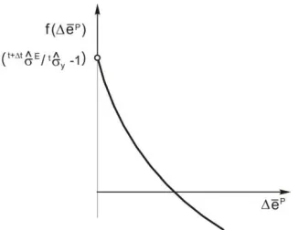
This function has a monotonic character (in Fig. 3 is shown the function for mixed hardening case (M. Kojic and K. J. Bathe 2005)) and it is straightforward to numerically find the zero of the function.
Fig. 3. Monotonic character of the effective stress function for mixed hardening metal plasticity.
Also, it is straightforward (with a certain algebra) to derive a consistent tangent constitutive matrix to be used in (5). The main idea is to find proper derivatives of deviatoric stresses with respect to strains, which must include the governing parameter ep. Hence, we have:
'p
i i
ij p
j j
e
S S
C
e e e
(25)
Derivatives
ep /ej can be obtained by differentiating (24) with respect to ej:
*
3 0
p E p
y p
j j j
f e e
G
e e e e
(26)
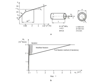
Fig. 4. Significance of use of the consistent tangent constitutive matrix. When elastic matrix CE is employed - 346 iterations were necessary to reach convergence, vs. only 2 iterations with the
consistent elastic-plastic matrix CEP (M. Kojic and K. J. Bathe 2005).
In summary, for a given total strains at end of time step and plastic strains at the start of (load) time step, the problem is reduced to find increment ep from (24). This equation is the basis for originally termed the “effective stress function” method; the procedure was introduced as a new concept in 1983. It was further generalized (as the governing parameter method (M. Kojic 1996)) to other material models in thermo-plasticity and creep of metals and in plasticity of geological materials, to all engineering physical conditions (2D, 3D, shells, beam and pipes); a summary is given in (M. Kojic and K. J. Bathe 2005). A number of Ph. D. and MS theses have been completed at Mech. Eng. Department of Univ Kragujevac, as, for exampe (R. Slavkovic 1986; I. Vlastelica 2002). The above straightforward steps show a beauty of the simple and robust procedure. It has been built into the ADINA code as well as into the PAK (M. Kojic et al. 2009) and has been used over decades for research and in industry.
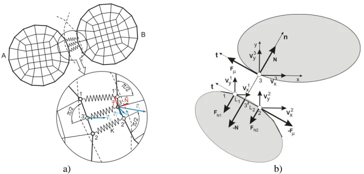
2.2 Contact problems
8
a) b)
Fig. 5. Modeling of contact between bodies by 1D elastic elements, 2D problems (V. Isailovic 2012). a) Interaction represented by forces between nodes and corresponding segments of the
bodies. b) Velocities, normal and tangential interaction forces at two bodies.
It is quite straightforward to find the current conditions of the adjacent (within a given range of the influence domain) nodes and segments during motion of bodies and calculate the interaction forces. For example, increment of normal forces on the segment 1-2 in Fig. 5b can be expressed in the form
1 1 2 2 3 3
1 x x 1 y y 2 x x 2 y y x x y y
N
k t h V n
h V n
h V n
h V n
V n
V n
(27)
where
2 1
1 2
1 2 1 2
,
L
L
h
h
L
L
L
L
and L1 and L2 are the distances along the segment measured from point 3‟ (the closest point of
segment to the node 3 of the adjacent body);
V
xIand
V
yI are nodal velocity increments;x
n
andn
y are components of the normal to the segment; and k the line element stiffness. From this basic equation, the appropriate corrections of stiffness matrices of the finite elements can be derived - for elements containing boundary nodes of both bodies (details not given here)This simple concept can be generalized to 3D conditions and to various characteristics of the contact, including nonlinearity, viscous effects, attractive and stochastic characters. It has been built into our FE code (M. Kojic et al. 2009) for the solid fluid interaction and has shown robustness and applicability to complex shapes of interacting bodies and multibody systems.
3. Solid-fluid interaction
a) Strong coupling (balance equations for solid and fluid form one system of equations and are solved simultaneously);
b) Remeshing procedure.
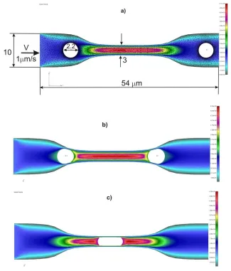
Although it requires significant computations and may be less efficient than other methods, this simplest and most straightforward approach gives the most reliable basis for detailed analyses of microcirculations (V. Isailovic 2012).
3.1. Motion of incompressible solids
Here is briefly described another simple and most straightforward concept of modeling motion of incompressible solids within incompressible fluid. These conditions are particularly important in microcirculation within living bodies. We emphasize that modeling of incompressible deformation of solids has been investigated by large number of authors (Raum K et al. 2006; D. Boffi et al. 2013) since it represents a challenge in computational mechanics.
Following the approach in modeling incompressible plastic deformation (Section 2.1) and fluid model in Section 1, it is natural to start with decomposition of stresses into deviatoric and mean parts according to (17). Then we can write the principle of virtual work in a weak form,
'
T v m T V
0
Ve
dV
e σ'
u f
(28)with separating deviatoric stresses and strains, and the mean stress and volumetric strain ev. The
FE balance equations can be further derived as usual (details are given in (M. Kojic et al. 2013)) and they have the same form as for fluid (10). Also, we employ the incompressibility condition (9) as for the fluid. Taking interpolation for the mean stress as for linear fluid elements (constant pressure over element), we have that the pressure-velocity matrix Kvp can be written
as
T vT
vp L
V
dV
K
B T
(29)where the matrix
T
v can be expressed in the formv
vn T
T
T
0
,T
vn
1 1 1
(30)10
Fig. 6. Motion of deformable disk (cell) within a channel, velocity field and disk shape. a) Geometrical data and FE mesh, with initial and final positions; b) Shape of the disk at the moments of entering and leaving the channel narrowing; c) Position of disk at the middle of the
channel. Material is viscoelastic.
3.2 Motion of rigid body within fluid
Here, we give a simple concept of modeling rigid body motion in fluid within the strong coupling methodology. Again, it is a straightforward derivation.
Fig. 7. Coupling motion of rigid body and fluid. Velocity of the common node J can be expressed by velocity of the center of mass C and angular velocity.
Considering velocity of the common node J of fluid and rigid solid, we can express this velocity in terms of velocity VC of the center of mass and angular velocity ω:
J C J C
C x y z
J J J
C C C
x
x
y
y
z
z
i
j
k
V
V
ω
r
r
V
(31)
Therefore, in calculating the element matrix and internal forces of the finite element, we simply impose transformations of the form:
T
K
T KT
,
TF
T F
(32)where the „bar‟ denotes transformed matrix and nodal force. The transformation matrix contains relative coordinates between points J and C, according to (31).
The author‟s simple concept of coupling rigid body motion with other deformable bodies has been implemented in ref. (Z. Bogdanovic 1998), and is analogous to this coupling rigid body motion with fluid flow. The above relations have been implemented in our code and solutions agree with the ones obtained by discretization of solid.
4. Multiscale diffusion and numerical homogenization algorithm
12
diffusion. It is of great interest to have proper computational methods which can capture transport of molecules (drug) and particles (drug carriers) in blood vessels and within tissue. Multiscale models, which couple events on molecular scale with those in larger domains (micron size) are necessary.
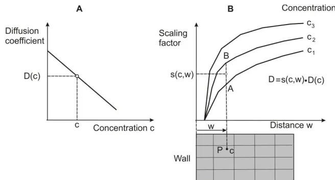
We here present one simple concept of coupling molecular dynamics (MD) and FE method in modeling of diffusion. It is natural to employ MD to calculate the effective diffusion coefficient and substitute it into the FE models according to equations (13) and (14). Calculation of the effective diffusion coefficient is performed using the “bulk” diffusion coefficient and scaling functions obtained by MD (illustration is shown in Fig. 8). By the scaling functions we take into account surface effects on motion of diffusing molecules.
Fig. 8. Evaluation of the effective diffusion coefficient using scaling functions obtained by MD (A. Ziemys et al. 2011; M. Kojic et al. 2011).
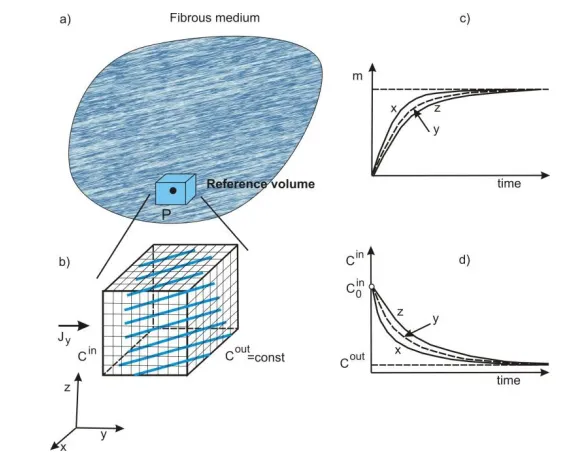
Detailed microstructural models, which take into account complex microstructure (as in case of diffusion within tissue), cannot be used in practical applications where larger domains (of millimeter size in case of tissue) since they will require enormous computational effort. It is desirable to have a macro-scale continuum model which captures the complex process within microstructure.
Fig. 9. Concept of numerical homogenization. Mass release curves within a reference volume (b) around point P (a) must be the same (c). In (d) is shown concentration at the inlet boundary
during diffusion through microstructure within microstructural model.
continuum and microstructural models. This simply is true because the mass flux is the same over the whole range of concentration,
( ) ( ) i
i i
dm
J tg
dt
(33)
where Ji is mass flux in direction xi and ( )i
14
Fig. 10. Diffusion within complex microstructure. a) Distribution od the diffusion coefficient
Dx; b) Distribution of flux in x-direction; c) Distribution of flux in x-direction for several planes
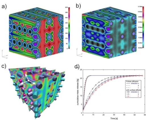
(a,b,c correspond to time 0.4sec); d) Mass release curves for x,y,z directions, solutions obtained using microstructural and continuum models. Details are given in ref. (M. Kojic et al. 2014).
5. Concluding remarks
It is demonstrated that simple concepts can produce very interesting results in computational mechanics. The author was lucky to work on various challenging topics and within stimulating environment, with people who inspired the efforts and contributed in elucidating problems to be solved. The author‟s approach was always to seek understanding the essence of the task and to try to find a simple way to resolve the problem. Several examples of success in this effort are selected.
Acknowledgments
A number of institutions contributed to this work over several decades, and here are listed just several: Mechanical Engineering Faculty Univ Kragujevac, Ministry of Science of Serbia, City of Kragujevac, Factory “Zastava” Kragujevac, ADINA R&D, Harvard School of Public Health, MIT-Mech. Eng. Department, Serbian Academy of Science and Arts, Houston Methodist Research Institute, R&D Center for Bioengineering, Kragujevac.
The author acknowledges the Serbian Ministry of Education and Science, grants OI 174028 and III 41007.
Једноставни концепти у рачунској механици – да ли они стварно
раде?
Милош Којић
Универзитет Метрополитан у Београду - Истраживачко развојни центар за биоинжењеринг у Крагујевцу, Првослава Стојановића 6, 3400 Крагујевац, Србија Houston Methodist Research Institute, The Department of Nanomedicine, 6670 Bertner Ave., R7-117, Houston, TX 77030
Резиме
Циљ овог рада је да прикаже неке од једноставних концепата уведених од стране аутора. Аутор је утврдио, после вишедеценијског рада у рачунској механици, да је (скоро увек) тачно да што је концепт једноставнији – методологија је општија и атрактивнија. Ради комплетности дат је кратак преглед основних релација и њихове одговарајуће формулације у методи коначних елемената (МКЕ). Области обухватају механику солида и флуида, биомеханику, поља физичких величина и мултискалну дифузију. Типични примери илуструју примену једноставних концепата. Све скупа, циљ овог рада би могао да буде мотивација за решавање проблема веће сложености на једноставан начин.
Кључне речи: Метод коначних елемената, интеракција солид-флуид, интеграција напона, мокроструктурно струјање флуида, деформисање нестишљивог солида.
References
M. Kojic, N. Filipovic, B. Stojanovic, N. Kojic, (2008). Computer Methods in Bioengineering – Theoretical Background, Examples and Software, J. Wiley and Sons.
K. J. Bathe, (1996). Finite Element Procedures, Prentice-Hall, Englewood Cliffs.
M. Kojic, R. Slavkovic, M. Zivkovic, N. Grujovic, (1998). Finite Eelement Method I – Linear Analysis, (in Serbian) Mechanical Eng. Faculty, Kragujevac.
N. Filipovic, (2011). The fundamentals of Bioengineering, (in Serbian) Mechanical Eng. Faculty, Kragujevac.
M. Kojic and K. J. Bathe, (2005). Inelastic Analysis of Solids and Structures, Springer.
M. Kojic, (1996). The governing parameter method for implicit integration of viscoplastic constitutive relations for isotropic and orthotropic metals, Computational Mechanics, Vol. 19, No. 1, pp. 49-57.
R. Slavkovic, (1986). Solution of Large Strain of a Continuum with Application in the Finite Element Method, Ph. D. Thesis, Mech. Eng. Dept. Univ. Kragujevac.
D. Begovic, (1995). Integration of Constitutive Equations in Case of Thermoplastic and Creep Deformation of Metals, MS Thesis, Mech. Eng. Dept. Univ. Kragujevac.
I. Vlastelica, (2002). Methods of Modeling of Elasto-Plastic Deformation of Non-Porous and Porous Metals in Fracture Mechanics, Ph. D. Thesis, Mech. Eng. Dept. Univ. Kragujevac. M. Kojic, R. Slavkovic, M. Zivkovic, N. Grujovic, N. Filipovic, (2009). PAK – Finite element
16
V. Isailovic, (2012). Numerical modeling of motion of cells, micro- and nano- particles in blood vessels. Information Tchnology. Metropolitan University, Belgrade.
J. C. Simo and M. S. Rafai, (1990). A class of assumed strain method and incompatible modes,
J. Numerical Methods in Engineering, 29, 1595-1638.
E. L. Wilson and A. Ibrahimbegovic, (1990). Use of incompatible displacement modes for the calculation of element stiffnesses and stresses, Finite Elements in Analysis and Design, 7, 229-241.
R. Slavkovic, M. Zivkovic and M. Kojic, (1994). Enhanced 8-node three-dimensional solid and 4-node shell elements with incompatible generalized displacements, Communications in Numerical Methods in Engineering, 10, 699-709.
J. A. Weiss, B. N. Maker and S. Govindjee, (1996). Finite element implementation of incompressible, transversely isotropic hyperelasticity, Comput. Methods Appl. Mech.
Engrg., 135, 107-128.
G. N. Gatica and E. P. Stephan, (2002). A mixed-FEM formulation for nonlinear incompressible elasticity in the plane, Numer. Methods Partial Differential Eq., 18, 105-128.
D. Boffi, F. Brezzi and M. Fortin, (2013). Mixed Finite Element Methods and Applications,
Springer Series in Computational Mathematics (Eds. R. E. Bank, R. L. Graham, J. Stoer, R. S. Varga and H. Yserentant), 44.
M. Kojic, Mixed formulation for incompressible solid within the FE method, with application to motion of solid in fluid, Publications of Department for Technical Sciences, Serbian Academy of Sciences and Arts, to be published.
Z. Bogdanovic, (1998). Modeling of statics and dynamics consisting of deformable and rigid bodies using FE method, MS thesis, Mech. Eng. Dept. Univ. Kragujevac.
A. Ziemys, M. Kojic, M. Milosevic, N. Kojic, F. Hussain, M. Ferrari, A. Grattoni, (2011). Hierarchical modeling of diffusive transport through nanochannels by coupling molecular dynamics with finite element method, Journal of Computational Physics, 230, 5722– 5731. M. Kojic, M. Milosevic, N. Kojic, M. Ferrari, A. Ziemys, (2011). On diffusion in nanospace, J.
Serbian Soc. Comp. Mechanics, Vol. 5, No. 1, 84-109.
M. Kojic, A. Ziemys, M. Milosevic, V. Isailovic, N. Kojic, M. Rosic, N. Filipovic, M. Ferrari, (2011). Transport in biological systems, J. Serbian Soc. Comp. Mechanics, Vol. 5, No. 2, 101-128.
M. Milosevic, (2012). Numerical Modeling of Diffusion within Composite Media. Ph. D. Thesis, Mech. Eng. Dept. Univ. Kragujevac.