Application of GAs to Determine the Parameters of a Time Series Model

(1)

Research article

Available online www.ijsrr.org

ISSN: 2279–0543

International Journal of Scientific Research and Reviews

Application of GAs to Determine the Parameters of a Time Series

Model

**Zouaoui Chikr El Mezouar* and Laid Gasmi**

Bechar University F.S.T Algeria.

ABSTRACT

We have witnessed in recent years a very rapid growth of work using genetic algorithms (GA). This trend can be observed in all areas of science economic. The aim of this article, we are interested in the application genetic algorithms for estimating the parameters of ARMA model (in the context of linear time series). To confirm the effectiveness of these new mechanisms, we apply both methods (the method of Box and Jenkins and her GA), to estimate the parameters of the model and compare the results obtained.

KEY WORDS -

Genetic algorithm, parameters; ARMA models; Time series; method of Box and Jenkins.

(2)

IJSRR, 4(1) Jan. – March. 2015 Page 32

INTRODUCTION : -

The study of time series or time series corresponds to the statistical analysis of observations

equally spaced in time. For the majority of these phenomena, there is often a dependence time

between observations, which have autoregressive modeling: the past is used to explain the present

and predict the future. Model and predict a time series is assumed in the most cases, to make

assumptions about its behavior using as it is non-deterministic series he’ll have the random

component "varies, but not too much." This condition will result in the "stationary "Which implies a

certain regularity of the process and allows deriving its asymptotic properties. When one has a series



Xt



in non-stationary stochastic, it should be modeled by a processARIMA p d q



; ;



, where d is the

order of differentiation (or integration).

Having successfully transformed these data, the problem is to find a satisfactory ARMA model

and particularly as to determine and to find the autocorrelation functions and autocorrelation

functions partial. The identification is mainly based on the analysis of the ACF (autocorrelation

function) and PACF (the partial autocorrelation functions) series considered.

The prediction method of Box-Jenkins1, 2 is particularly well suited to the treatment of series

complex historical and other situations in which the Basic Law is not immediately apparent.

However, as she deals with much more complicated situations, it is difficult to grasp the principles

of this technique, as well as the limits of its application. In addition, the cost of me- Box-Jenkins

method in a given situation is usually much higher than that of all other quantitative methods. We

know that the applications of genetic algorithms are multiple: Medicine3, robotics 4, analysis of time

series 5, 6, image processing 7

Our application examples helped us realize that the coding of data for model a problem is

complex. On the other hand, we also saw difficulties effectively choose good parameter for the

various operators (mutation, crossover, selection, replace placement). Choices in relation to the

operators themselves are also manageable, knowing that some are most appropriate to the problem

and let correlation means that they optimizer.

APPLICATION

We will study two sets of simulated and the other with real data by two methods-Box

(3)

Modeling the simulated series (B-J)

Begin with a series of simulated autoregressive process (2), 300 observations. Table 1 gives

the coefficients of the model8,9,10.

The graphic (1): Series

_{ }

Y_t and the series (Yt adjusted) adjusted by the model, shows the absence of

a net difference between the two curves (we see a good fit).

Figure 1 - and Ytadjusts

To validate the model we are going to study the residues (Table2). Coefficient(s) Estimate Std. Error

1 1.5572 0.03665

2 -0.76809 0.03658

Table 1 Coefficient model AR (2) of the series

Table 2 Tests on residue

Test Formula p -value

Kolmogorov-Smirnovles lillie:test(residus) 0.08785

Student t test(residus;mu = 0; conf:level = 0:95) 0.4671

(4)

Modeling the simulated series (AG)

Now to the second method (Genetic Algorithm). it various the number of observations, the size of the initial population (solutions



i) number of iteration of the algorithm genetic, crossover

probability (from 1% to 100%) mutation probability (from 1% to 100%) and stop criterion ( mse is

minimum). (



₁and



₂) Best, we got was (according to Table 3):



1, 2

 

1.5619365334 , 0.7727730311



Best     ), mse1.6944448763. The adjusted this model

(GA) series is stationary over we see no difference between the two chronics (Figure 2).

Figure 2 Yt and Yt ajus AG

This allows us to conclude that the residues form a white noise (Table 4), where model validation.

We can have confidence in our predictions.

Table 3. The conditions for obtaining the best result (



₁and



₂)

NBOBSERVATIONS = 298 number of observations NBITERATIONS = 290 the initial population size

NBITERATIONS = 100 Iteration number of genetics algorithm

PROBCROISEMENT =90% crossing probability

PROBMUTATION = 10% probability of mutation

0.000001

  stop criterion : mse

Table 4 Tests on residue

(5)

The graphic (3) Summarizes the quality of prediction and hence the performance of both models.

Figure 3 Performance of the two models GA & BJ

Visually, we see no difference between the two models. But the measures contained in the table(5),

give preference to the model of Box and Jenkins.

MAPE MSE

B-J 1.158333 1.231707

GA 1.160062 1.233228

This time we discuss a real series, which represents the number of car accidents (weekly) for

the years 1992 and 1995. We have 140 observations (source : Department of Statistics and O R

,Faculty of science, Kuwait University)14.

Modeling and Prediction of the real series (number of car accidents)

1.1 Method B- J

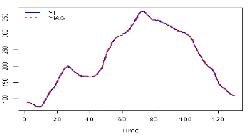
The graphic (4) Series, which represents the number of car accidents (weekly) for the years 1992 and

(6)

Figure 4 Yt , ACF,PACF

After the two transformations : Lt = log(Y t) and DL = diff(Lt) = diff(log(Y t)) we obtain a

stationary series (DL) : p - value = 0:02066 test (adf.test). Best suited to this model is



2;1;0



ARIM . Table (6) gives the coefficients of the model14.

Move on to the adjustment of our series by this model. According to the graphic (5), there is no

differentiation between the two series.

Figure 5 The adjustment of the series by this model (ARIMA (2; 1; 0))

Coefficient(s) Estimate Std. Error

1 1.4139 0.0767

2 -0.4827 0.0772

(7)

To validate the model we will study the residues.

This allows us to conclude that the residues form a white noise (Table7), where model validation.

We can have confidence in our predictions.

1.2 Method AG

Best



₁and₂



, Which was obtained under the conditions (8):



 1, 2

 

 1.3623294021, 0.4199999997



The adjusted by the model and the real series are graphically almost identical graphic (6)

Table 7 Tests residues

Ljung - Box Box.test(residus; lag = 50; type = "LjungBox") 0.9477

Table 8 The conditions for obtaining the best result



₁and₂



NBITERATIONS = 1000 the initial population size

NBITERATIONS = 100 nombre d’iteration of genetics algorithme

PROBCROISEMENT =90% crossing probability

PROBMUTATION = 10% probability of mutation

0.000001

(8)

Table 9 Tests residues

Ljung - Box Box.test(residus; lag = 50; type = "LjungBox") 0.6273

This enables us to conclude that the residues form a white noise (Table 9), where model validation.

The graphic (7) summarizes the quality of prediction and hence the performance of both models.

Figure 7 Performance of both models AG & BJ

Visually, there is a clear difference between the qualities of predictions, where the second validation

method (GA).

Table 11 conclusion of comparison

MAPE MSE

B-J 1.158333 1.231707

GA 1.160062 1.233228

CONCLUSIONS

The first inspiration and driving force of this study were convinced that the sharing of

experiences and knowledge between different fields of knowledge are an essential element of this

enrichment even knowing . In the experimental part, we found that the use of GA Allow to obtain

very good results in comparison with the results given by the method of Box Jenkins ( in particular ,

for the actual chronic ). Therefore, the conclusion of this study is not only proposal to continue the

way of using Genetic Algorithms in the field of time series ( parameter estimation ), and thus predict,

(9)

they provide fairly quickly an acceptable solution. Nevertheless, it is possible to improve effectively

enough by combining it with a deterministic algorithm.

REFERENCES

1.

Box P., Jenkins G. M. Time series analysis: Forecasting and control. San Francisco, CA:

Holden-day Inc; 1976.

2.

Jean M. V., Reto G. Model selection using a simplex reproduction genetic algorithm. Signal

Processing. 1999; 78: 321-327.

3.

Yang, G., Reinstein, L.E., Pai, S., Xu, Z., Carroll, D.L., A new genetic algorithm technique in

optimization of prostate implants, accepted for publication in the Medical Physics Journal,

1998.

4.

Zalzala, A.M.S. and Fleming, P.J., Genetic Algorithms in Engineering Sytems, p161-202,

IEE, London, 1997.

5.

Mahfoud, S.W. and Mani, G., Financial forecasting using genetic algorithms, Applied

Artijicial Intelligence, 1996; 10: 543-565,.

6.

Packard, N. H., A genetic learning algorithm for the analysis of complex data, Complex

Systems, 1990; 4(5):543412,

7.

Chen, Y.W.,N akao, Z., Arakaki, K., Tamura, S., Blind deconvolution based on genetic

algorithms, IEICE Transactions on Fundamentals of Electronics, Communications and

Computer Sciences. 1997; E80A (12): 2603-2607.

8.

Akaike H., Fitting autoregressive models for prediction, Ann. Inst. Stat. Math. 1969; 21:

243-247.

9.

Engle R.F. Autoregressive conditional heterocedasticity with estimates of the variance of

UK inflation, Econometrica. 1982; 50: 145-157.

10.

Commandeur J. J. F., Koopman S. J. An Introduction to State Space Time Series Analysis.

Oxford, New York; 2007.

11.

Dickey D.A. et Fuller W.A., Distribution of the estimators for autoregressive time series with

a unit root, J. Amer. Stat. Soc. 1979; 74: 427-431.

(10)

13.

Sharpe, W.. Capital asset prices: A theory of market equilibrium under conditions of risk.

Journal of Finance. 1964; 19: 425–442.

14.

M. Gabr,Time Series Analysis Stat, Department of Statistics & O R, Faculty of science,