Detecting And Controlling Insect Vectors In Urban Environments: Novel Bayesian Methods For Complex Spatial Data

University of Pennsylvania

ScholarlyCommons

Publicly Accessible Penn Dissertations

2017

Detecting And Controlling Insect Vectors In Urban

Environments: Novel Bayesian Methods For

Complex Spatial Data

Erica Billig

University of Pennsylvania, [email protected]

Follow this and additional works at:

https://repository.upenn.edu/edissertations

Part of the

Epidemiology Commons

, and the

Statistics and Probability Commons

This paper is posted at ScholarlyCommons.https://repository.upenn.edu/edissertations/2193

For more information, please [email protected].

Recommended Citation

Billig, Erica, "Detecting And Controlling Insect Vectors In Urban Environments: Novel Bayesian Methods For Complex Spatial Data" (2017).Publicly Accessible Penn Dissertations. 2193.

Detecting And Controlling Insect Vectors In Urban Environments: Novel

Bayesian Methods For Complex Spatial Data

Abstract

Efforts to control the spread of vector-borne diseases often focus on the vector itself. Here, we develop novel

methods to strategically guide the search for vectors over urban landscapes. The methodology is motivated by

Triatoma infestans, the vector of Chagas disease, a re-emerging vector in Arequipa, Peru. We first propose a

novel stochastic epidemic model that incorporates both the counts of disease vectors at each observed house

and the complex spatial dispersal dynamics. The goal of our analysis is to predict and identify houses that are

infested with T. infestans for entomological inspection and insecticide treatment. A Bayesian method is used

to augment the observed data, estimate the insect population growth and dispersal parameters, and determine

posterior infestation probabilities of households. We investigate the properties of the model through

simulation studies and implement the strategy in a region of Arequipa by inspecting houses with the highest

posterior probabilities of infestation and report the results from the field study. After piloting this model in the

field and assessing the strengths and weaknesses, we propose a much faster method that extends a Gaussian

Field (GF) model to incorporate the urban landscape. GF models can be used to create risk maps of vector

presence across large urban environments. However, these models do not typically account for the possibility

that city streets function as permeable barriers for insect vectors. We extend GF models to account for this

urban landscape. We demonstrate our method on simulated datasets and then apply it to data on T. infestans.

We estimate that streets increase the effect of distance on the probability of vector presence at least 1.5 fold

compared to the undivided environment. Lastly, we propose a Bayesian generalized multivariate conditional

autoregressive approach to jointly model the distribution of vectors, T. infestans, with the proportion of

vectors that carry the parasite of Chagas disease, Trypanosoma cruzi. We demonstrate the properties of the

model using simulation studies, and apply the method to data from Arequipa.

Degree Type

Dissertation

Degree Name

Doctor of Philosophy (PhD)

Graduate Group

Epidemiology & Biostatistics

First Advisor

Jason A. Roy

Second Advisor

Michael Z. Levy

Keywords

Subject Categories

DETECTING AND CONTROLLING INSECT VECTORS IN URBAN ENVIRONMENTS: NOVEL BAYESIAN METHODS FOR COMPLEX SPATIAL DATA

Erica Marie Weinmann Billig

A DISSERTATION

in

Epidemiology and Biostatistics

Presented to the Faculties of the University of Pennsylvania

in

Partial Fulfillment of the Requirements for the

Degree of Doctor of Philosophy

2017

Supervisor of Dissertation Co-Supervisor of Dissertation

Jason A. Roy Michael Z. Levy

Associate Professor of Biostatistics Associate Professor of Epidemiology

Graduate Group Chairperson

Nandita Mitra, Professor of Biostatistics

Dissertation Committee

Michelle E. Ross, Assistant Professor of Biostatistics

Ricardo Castillo Neyra, Scientific Director, Universidad Peruana Cayetano Heredia

DETECTING AND CONTROLLING INSECT VECTORS IN URBAN ENVIRONMENTS: NOVEL

BAYESIAN METHODS FOR COMPLEX SPATIAL DATA

c

COPYRIGHT

2017

Erica Marie Weinmann Billig

This work is licensed under the

Creative Commons Attribution

NonCommercial-ShareAlike 3.0

License

To view a copy of this license, visit

ACKNOWLEDGEMENT

The writing of this dissertation would not have been possible without the support and insight of

many others. I would first like to thank my advisors, Dr. Jason Roy and Dr. Michael Levy, for their

dedication, advice, patience, and guidance over the years. I am grateful that even though they

had not worked together before, they agreed to co-advise me. They spent much time and energy

working with me on my dissertation, and were patient and kind as I made mistakes. Every time I

reached an obstacle, they helped me find a way to a solution. I truly believe that because of them,

I have continued to enjoy working on this project.

I would also like to thank my committee, Dr. Michelle Ross, and Dr. Ricardo Castillo Neyra, for

their ideas and help along the way. Dr. Ross met with me frequently to teach me spatial statistics.

She had insights that yielded results included here. Dr. Castillo Neyra knows these data better

than anyone, and he readily answered my questions that helped me understand the content of the

project. I especially want to thank the late Dr. F. Ellis McKenzie, with whom I worked for two years at

the Fogarty International Center at NIH. He was a wise and thoughtful mentor, a brilliant scientist,

a role model, and initial member of my committee. Although he was not able to see the final result,

this dissertation bears his mark. His influence is evident not only here, but through the work of his

many students.

I would like to thank Dr. Christopher Hunter and the support of the Parasitology Training Grant,

5T32AI007532. The grant has allowed me to focus my time on my dissertation, and supported

me to present the results at several conferences. I would like to thank the team in Peru that has

spent so much time collecting, managing, and studying these data : Ministerio de Salud del Per ´u

(MINSA), the Direcci ´on General de Salud de las Personas (DGSP), the Estrategia Sanitaria

Na-cional de Prevenci ´on y Control de Enfermedades Metax ´enicas y Otras Transmitidas por Vectores

(ESNPCEMOTVS), the Direcci ´on General de Salud Ambiental (DIGESA), the Gerencia Regional

de Salud de Arequipa (GRSA).

I would like to thank the faculty, staff, and students at the University of Pennsylvania in the

Depart-ment of Epidemiology and Biostatistics. I am especially grateful to Dr. Justine Shults, Dr. Mary

Sammel, Dr. Mary Putt, and Dr. Scarlett Bellamy, who provided me with invaluable guidance and

presented in Chapter 3. I feel very fortunate that my graduate education has enabled me to connect

with many wonderful mentors, colleagues, and friends.

Lastly, I would also like to thank my family and friends, who were so supportive as I have pursued

my PhD. My parents, Dr. Gail Weinmann and Dr. Nathan Billig, have instilled in me a love of

science, and continued to encourage me to find a way to reach my potential. My fianc ´e, Jason

Rose, has been by my side since I began at Penn, and has always encouraged and believed in me,

ABSTRACT

DETECTING AND CONTROLLING INSECT VECTORS IN URBAN ENVIRONMENTS: NOVEL

BAYESIAN METHODS FOR COMPLEX SPATIAL DATA

Erica Marie Weinmann Billig

Jason A. Roy

Michael Z. Levy

Efforts to control the spread of vector-borne diseases often focus on the vector itself. Here, we

develop novel methods to strategically guide the search for vectors over urban landscapes. The

methodology is motivated byTriatoma infestans, the vector of Chagas disease, a re-emerging

vec-tor in Arequipa, Peru. We first propose a novel stochastic epidemic model that incorporates both

the counts of disease vectors at each observed house and the complex spatial dispersal

dynam-ics. The goal of our analysis is to predict and identify houses that are infested with T. infestans

for entomological inspection and insecticide treatment. A Bayesian method is used to augment

the observed data, estimate the insect population growth and dispersal parameters, and determine

posterior infestation probabilities of households. We investigate the properties of the model through

simulation studies and implement the strategy in a region of Arequipa by inspecting houses with the

highest posterior probabilities of infestation and report the results from the field study. After piloting

this model in the field and assessing the strengths and weaknesses, we propose a much faster

method that extends a Gaussian Field (GF) model to incorporate the urban landscape. GF models

can be used to create risk maps of vector presence across large urban environments. However,

these models do not typically account for the possibility that city streets function as permeable

bar-riers for insect vectors. We extend GF models to account for this urban landscape. We demonstrate

our method on simulated datasets and then apply it to data onT. infestans. We estimate that streets

increase the effect of distance on the probability of vector presence at least 1.5 fold compared to

the undivided environment. Lastly, we propose a Bayesian generalized multivariate conditional

au-toregressive approach to jointly model the distribution of vectors,T. infestans, with the proportion

of vectors that carry the parasite of Chagas disease, Trypanosoma cruzi. We demonstrate the

TABLE OF CONTENTS

ACKNOWLEDGEMENT . . . iii

ABSTRACT . . . v

LIST OF TABLES . . . viii

LIST OF ILLUSTRATIONS . . . x

CHAPTER 1 : INTRODUCTION . . . 1

1.1 Vector-borne diseases . . . 1

1.2 Motivation: Chagas disease . . . 1

1.3 Statistical background and developments . . . 2

CHAPTER 2 : REAL-TIMEEPIDEMIOLOGICALSEARCHSTRATEGY . . . 6

2.1 Introduction . . . 6

2.2 Methods . . . 7

2.3 Simulations . . . 17

2.4 Data Results . . . 18

2.5 Discussion . . . 20

CHAPTER 3 : RISK MAPS FOR CITIES: INCORPORATING STREETS INTO GEOSTATISTICAL MODELS . . . 23

3.1 Introduction . . . 23

3.2 Methods . . . 24

3.3 Simulations . . . 30

3.4 Data Results . . . 34

3.5 Discussion . . . 37

CHAPTER 4 : GENERALIZEDMULTIVARIATECONDITIONALAUTOREGRESSIVEMODEL FOR VECTOR-BORNEDISEASEDATA . . . 39

4.2 Methods . . . 41

4.3 Simulations . . . 47

4.4 Data Results . . . 48

4.5 Discussion . . . 50

CHAPTER 5 : DISCUSSION. . . 55

5.1 Conclusions . . . 55

5.2 Limitations . . . 57

5.3 Future directions . . . 58

APPENDICES . . . 62

LIST OF TABLES

TABLE 2.1 : Simulation results. Each estimate represents the mean of given quartile for the set of 200 replicates. We use the median estimate to verify our approach obtains accurate parameter estimates and report the median AUC of each

parameter set. . . 18

TABLE 3.1 : Description of map distortion in Figure 3.1 scaled so the spatial unit is the average distance between nearest neighbors on the same block. Interpre-tation ofS varies by specific map due to variability in sizes and shapes of city blocks. S describes ratio of distance between geographic median of each city block relative to the true map (which is equivalent toS= 1). Table summarizes how this distortion corresponds to additional distance between houses on different blocks using mean and standard deviation (sd). The distortion varies block by block due to irregular grid. . . 29

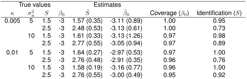
TABLE 3.2 : Results from 100 Monte Carlo simulations for each parameter set. The pa-rameter estimates are shown with the corresponding estimated standard deviations with the true values set for the simulations. The coverage of (βˆ0) is the average rate that the credible interval captures the true value ofβ0for identified simulation cases. The last column is the proportion of identifiable simulated datasets. . . 31

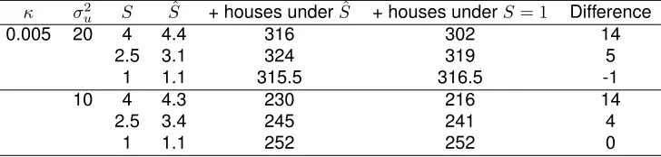
TABLE 3.3 : Difference in number of positive houses in the top 30% of probabilities of infestation using our approach of map distortion compared to using the true map with no distortion (S= 1). Model fit with true values ofS= 1,S= 2.5, andS = 4 when a randomly selected one-third of points were observed. Intercept fixed atβ0=−5. 100 simulated datasets were run at each value. We report number of positive houses in the top 30% of probabilities which were treated as unobserved (ie. no gain for houses that were observed as positive). . . 33

TABLE 4.1 : Median estimates with median of the 95% credible interval of 40 simulated datasets. . . 48

TABLE 4.2 : Data results using three models (Eq. 4.1, 4.2, 4.3). The full model allows all parameters to vary. The partial model allowsη20 andη30 to vary, but fixes η21 = 0andη31 = 0. The independent model fixes all linking parameters, η= 0. In all models, covariables are the same: βi0 corresponds to the model intercept,βi1 is the estimated effect of guinea pigs (cuy),βi2 is the estimated effect of dogs,βi3is the estimated effect of poultry,βi4estimates the effect of the presence of housing materials that are good habitats for vectors, andβi5 estimates the effect of the presence of housing materials that are poor habitats for vectors fori= 1,2,3. Coefficient credible intervals of covariables that did not contain 0 are highlighted in red. . . 50

TABLE B.1 : Simulation results with the variation in interceptβ0. . . 65

TABLE B.2 : Simulation results with the variation in interceptκ. . . 66

TABLE B.3 : Simulation results with the variation in interceptβ0. . . 66

LIST OF ILLUSTRATIONS

FIGURE 2.1 : ROC curves describing the ability of the RJMCMC to uncover unreported infestations in a simulated vector-borne epidemic. In each simulation, 1/3 of infestations were randomly removed to recover. 50 randomly selected ROC curves of each parameter regime are shown. (a){β, r}={0.02,1.6} (b){β, r}={0.7,1.8}(c){β, r}={0.3,2.1} . . . 18 FIGURE 2.2 : Posterior estimate ofβ, the probability of successful invasion of a migrating

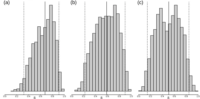
bug, at the beginning of the inspection campaign in each community, indi-cating median and 95% credible interval of RJMCMC chains: (a) Commu-nity 1: 0.67 (0.33, 0.91) (b) CommuCommu-nity 2: 0.59 (0.22, 0.90) (c) CommuCommu-nity 3: 0.51 (0.15, 0.85) . . . 19 FIGURE 2.3 : Path of inspectors in study region from October 2015 through December

2015. Sites of attempted inspections (blue circles) and successfully in-spected houses (black circle) shown, as well as daily routes (blue lines). Previous confirmed infestations (red plus signs) also shown. Points are jittered to de-identify data. . . 20

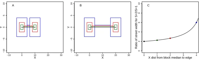
FIGURE 3.1 : A)S = 1, which corresponds to the true map of section in Mariano Mel-gar, Arequipa, Peru used for simulations. There is no map distortion at this scale. B) Distorted map to a scale ofS = 1.5, where the distance be-tween geographic medians of blocks are 1.5 fold the true distance. C) Map distorted to scaleS = 2.5, where distance between geographic medians of blocks are 2.5 fold the true distance. Note distance between houses within block is maintained but distance between houses on different blocks is stretched. . . 27 FIGURE 3.2 : In this figure, we demonstrate how streets between larger blocks result in

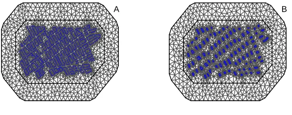
a larger barrier effect. A. Four hypothetical blocks super-imposed. The smallest block is simply one house. The largest block has an X distance of 4 from the block median to the edge of the block. B. Same hypothetical blocks after distortion with S = 2. C. The ratio of street width for this distortion atS = 2 compared to no distortion atS = 1. The street width doubles if the block is a single house and the distance from block median to edge is zero. Otherwise, the street width more than doubles, and the effect increases as the block size increases. . . 29 FIGURE 3.3 : Mesh over the map of the simulation region (houses in blue). Maximum

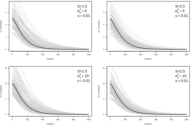
edge length is constrained to 100S to keep meshes consistent between scales. A.S= 1B.S= 1.5 . . . 30 FIGURE 3.4 : Comparing the estimated Mat ´ern covariance function (gray) with the true

Mat ´ern covariance function (black) under four parameter sets. . . 32 FIGURE 3.5 : Three unidentifiable and identifiable log-likelihoods and the

correspond-ing simulated datasets. Unidentifiable landscapes were uncommon, (rates varied based on the true parameter values ofκandσ2

u) and in most cases

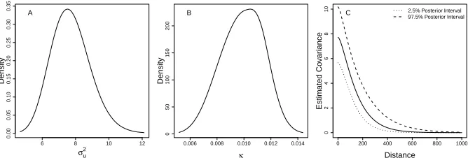
FIGURE 3.6 : Map of the study region, the district of Mariano Melgar, Arequipa, Peru, which consists of 12,069 houses and 724 blocks. Color corresponds to number of known infested houses on the block. . . 35 FIGURE 3.7 : Posterior distributions of estimated parameters when S = 1.5. A.

Poste-rior distribution ofσ2

uB. Posterior distribution of κ. C. Estimated posterior

distribution of Mat ´ern covariance, as a function of distance. For reference, when the map is scaled toS= 1.5, the average distance between nearest neighbors on the same block is 10.2 (sd= 5.5) and the average distance between nearest neighbors on different blocks is 62.4. (sd= 18.0) . . . 36 FIGURE 3.8 : Risk map of predicted probabilities of infestation using A)S = 1(true map)

B)S= 1.5and C)S = 3. The last panel shows differences in risk between scales of the area enclosed in the black rectangle in more detail. The color scale showsP(infestation)and ranges from 0.74 (red) to 0.00 (purple) . . 37

FIGURE 4.1 : Data used in analysis. Dataset contains 577 sites (contained within 67 houses; house level data not shown). Sites with vectors (red) and number of vectors (size of point on log scale) shown with number of vectors that tested positive forT. cruzi(size of yellow point on log scale). . . 40 FIGURE 4.2 : Unfilled gray points indicate all sites. (a) Expected probability of vector

presence at each site (size of red point relative to gray point) (b) Expected count of vectors, conditional on the probability of vector presence (size proportional to log count) (c) Expected proportion of positive vectors, con-ditional on expected vector distribution (size of gold point relative to red point). Red point is relative to the size of the log of the number of observed

T. infestansat that site. . . 52

FIGURE A.1 : Bounded growth using the Beverton-Holt model compared to unbounded growth. Difference in slopes at time of new infestation was incorporated into hazard function to quantify infestation severity into the probability of infesting a neighboring house. . . 62 FIGURE A.2 : Ranking of each house across 3 RJMCMC chains. There were a few

houses that changed significantly, but most houses remained within a few rankings between chains. We use the median ranking between chains to give inspectors. . . 63 FIGURE A.3 : Ranking of each house across 5 potential carrying capacities. There were

a few houses that changed significantly, but most houses remained within a few rankings between carrying capacity values. . . 64

FIGURE B.1 : Log-likelihood analysis across different scales, S. In most cases, S is clearly identifiable, but in some cases (red rectangles) it is not. . . 67 FIGURE B.2 : Log-likelihood analysis across different scales,S. Likelihood is maximized

CHAPTER 1

I

1.1. Vector-borne diseases

Vector-borne diseases are increasingly common in urban areas, and efforts to control these

dis-eases are often targeted at the vector itself. However, detecting populations of disease vectors in

large urban environments is especially complex (Weaver, 2013, Knudsen and Slooff, 1992). Poor

and unplanned urban environments can create ideal breeding grounds for many vectors, facilitating

increased transmission of vector-borne diseases in population dense areas (Knudsen and Slooff,

1992, Bowman et al., 2008, Levy et al., 2006). Several arboviruses, including Dengue,

Chikun-gunya, West Nile, and Zika, have emerged repeatedly in urban areas (Haley, 2012, Sikka et al.,

2016). Parasitic diseases, such as malaria and Chagas disease, once considered rural problems,

have become common in cities (LaDeau et al., 2015, Delgado et al., 2013). In this dissertation, we

develop methods for real-time surveillance of the re-emerging vector of Chagas disease,Triatoma

infestans, in Arequipa, the second largest city in Peru.

1.2. Motivation: Chagas disease

Chagas disease has long been endemic in Central and South America and is caused by the parasite

Trypansoma cruzi (Mathers, Fat, and Boerma, 2008, Bern, 2015, Rassi and Marin-Neto, 2010).

Once infected with the parasite, the host will first suffer from the acute phase of the disease, which

presents symptoms like that of the flu. Infected individuals may suffer symptoms such as fever,

swollen lymph nodes, and, rarely, the classic sign of Chagas, Romana’s sign, where the periorbita

becomes inflamed (Bern, 2015). The acute phase typically lasts 4-8 weeks, at which point the

disease enters the chronic phase. During this phase, the patient is unlikely to have symptoms.

Approximately 20-30% of individuals in this phase will suffer a cardiac event over the course of a

lifetime, while others will enter a symptomatic chronic phase, which affects the nervous, digestive,

and cardiac systems (Bern, 2015). One of the challenges of assessing the burden of Chagas

disease lies in the complex and wide range of symptoms. Patients often go undiagnosed and

An estimated 5.7 million people are currently living with Chagas disease (Bern, 2015). The

preva-lence has dropped substantially over the last few decades, largely due to a successful public health

campaign to control vector populations (Dias, Silveira, and Schofield, 2002). Arequipa has only one

vector ofT. cruzi transmission,T. infestans, a species of triatomine that thrives in urban settings.

The species prefers environments such as guinea pig pens, common in Peru, and housing

materi-als with dark cracks and crevices (Levy et al., 2006). Since the insect rarely flies, there is a highly

spatial aspect to the observed vector distribution patterns. Previous studies have shown that the

vectors are much more likely to move within city blocks than cross a street (Barbu, Dumonteil, and

Gourbi `ere, 2010, Barbu et al., 2013).

To control the spread of Chagas disease, Arequipa began an inspection and spray campaign to

target T. infestans in 2003 (Barbu et al., 2014). During the first phase of the campaign,

prelimi-nary inspections were conducted on a locality level, followed by a treatment phase during which

insecticide was applied to the targeted areas. These phases were followed by surveillance, during

which residents report infestations, which are followed-up by an inspection to that location, and

surrounding locations if a true vector is found. From the spray campaign and subsequent

surveil-lance, detailed data was collected on vector prevalence, including the date, location, and number

of vectors observed at houses throughout the city. We are motivated to use this data to guide a

new campaign to target the vectors that have re-emerged since the initial campaign – we want to

inspect high risk houses for vectors, and update the risk as inspections are completed.

Here, we develop methods to search urban environments for disease vectors, and apply them to the

ongoing efforts to eliminate the spread ofT. infestans, in Arequipa, Peru. Different from other types

of search strategies, where the coveted item is not moving or spreading, controlling the spread of

disease vectors in real time requires identifying and treating infested households before they move

or infest others. We also present a method to estimate the proportion of vectors infected with T.

cruzi, conditional on the distribution ofT. infestans. Our methods expand upon existing Bayesian

spatial, temporal, and epidemic modeling tools.

1.3. Statistical background and developments

In the second chapter, we propose a novel stochastic compartmental model to estimate the

in Arequipa, to guide our inspection strategy. Stochastic epidemic models are a popular tool to

describe the course of an infectious disease epidemic. Using this approach, we treat the spread

ofT. infestansthrough houses in the city like an infectious disease spreading through a population

of individuals. Fitting stochastic epidemic models to data is challenging due to the detailed data

necessary to retain a tractable likelihood (Andersson and Britton, 2012). We use a

susceptible-infected-removed (SIR) model: every house in the system is in one of these three states

(suscep-tible, infected, or treated) at any given time point, and parameters describe the rates of transition

between states. However, the likelihood of this model includes the time of infestation and treatment

of every house (Becker, 1989). In practice, we do not observe the true infestation time of each

house, and many houses in the system have never been inspected. O’Neill et al. developed an

approach to augment the data and retain a tractable likelihood when the infestation times and total

number of infested houses are unobserved (O’Neill and Roberts, 1999). His key development is the

use of a reversible-jump Markov chain Monte Carlo, an estimation algorithm used when the number

of parameters is unknown. In this case, the total number of infested houses is unknown, and thus

there is an unknown number of unobserved infestation times, which are treated as parameters in

the model.

We expand off more recent methods, Jewell et al., 2009a and Jewell et al., 2009b, that incorporate

the ‘notification time’ of the house, or the time that the house is observed as infested into O’Neill’s

approach. Jewell’s method uses a susceptible-infected-notified-removed (SINR) model and

there-fore has additional parameters to capture the transition from the infected to notified, and notified to

removed, states of the system. The approach was developed in the context of notifiable diseases,

and the critical assumption necessary for a tractable likelihood of the SINR model, is a known

distribution that captures the true infestation time as a function of the later, observed notification

time. Due to the nature of how our data was collected, as part of both the spray campaign and

subsequent surveillance, we cannot make that key assumption.

We incorporate a house-level vector population growth model and use the counts of disease

vec-tors at each observed house to estimate the unobserved infestation time, by assuming houses with

more observed insects were infested less recently than houses with fewer insects. In addition,

we attempt to capture the complex spatial dispersal dynamics by using a kernel that incorporates

are infested withT. infestansfor entomological inspection and insecticide treatment. Our Bayesian

method is used to augment the observed data, estimate the insect population growth and

disper-sal parameters, and determine posterior infestation probabilities of households. We investigate

the properties of the model through simulation studies. We implement the strategy in a region of

Arequipa by inspecting houses with the highest posterior probabilities of infestation and report the

results from the field study. After implementing this model in the field, we identify strengths and

weaknesses of this approach. While the model captures the spatial heterogeneity and dynamic

movement of the vectors, the reversible-jump Markov chain Monte Carlo used for estimation is

computationally intensive and does not consistently converge quickly enough for real-time updates.

In the third chapter, we are motivated to develop a model to improve upon the weaknesses we

en-countered in our field implementation, including speed of convergence, while estimating the effect

of the urban landscape on the vector distribution. We use Gaussian field (GF) model, a type of

spatial model used for point-process, or geostatistical, data. Recent advances, both in theory and

computation, have enabled fast parameter estimation using this approach. Lindgren et al. found

a link between the GF and Gaussian Markov Random Field (GMRF) with the use of the Mat ´ern

covariance function, popular for geostatistical data (Lindgren, Rue, and Lindstr ¨om, 2011). Using

this link, we can estimate the parameters of the Mat ´ern covariance function using nested integrated

Laplace approximations. Rue et al. developed a sophisticated R package, ‘INLA’, to implement

this estimation algorithm, an alternative to Markov chain Monte Carlo, greatly easing the speed and

computational burden (Rue, Martino, and Chopin, 2009). Using a GF, we assume the observed

vector distributions are a realization of a stochastic process that is occurring over the landscape.

However, the GF assumes the process is occurring over a continuous, smooth, space, but the city

streets of the urban landscape create barriers for vector dispersal. Unlike true barriers, vectors

can cross city streets, but previous studies have shown thatT. infestansare more likely to move a

given distance within a city block than between city blocks (Barbu et al., 2013). We propose using

an additional parameter to capture the heterogeneity of the city landscape, by effectively distorting

the city map and widening the streets by an estimated distance, creating permeable barriers. Our

approach fits into the existing estimation software, making it accessible for researchers across

dis-ciplines, and easy to apply to different districts of Arequipa while maintaining the ability to regularly

update the model for ‘real-time’ estimation. Including the spatial structure of city streets may more

developing effective public health interventions to reduce transmission in population dense areas

(Weaver, 2013). We demonstrate our method on simulated datasets and then apply it to data on

Triatoma infestans, the principal vector of Chagas disease in Arequipa Peru.

In the fourth chapter, we develop a multivariate spatial model to study the proportion of vectors

infested with the parasite,T. cruzi, conditional on the count and spatial distribution of the population

of vectors themselves. In this approach, we build off of the traditional conditional autoregressive

(CAR) spatial model (Besag, 1975). Jin et al. developed a bivariate generalized conditional

autore-gressive model that uses linking parameters to create dependencies between spatial models (Jin,

Carlin, and Banerjee, 2005). We extend this model to link three CAR models: a logistic model of

the proportion ofT. cruziinfected vectors, and the two pieces of the zero-inflated Poisson mixture

model of the vector distributions. This approach has an inherent order in the structure and

inter-pretation. We first model the probability of vector presence, including a spatial random effect. We

then model the count of vectors, with a different spatial random effect, conditional on the probability

of vector presence. These two models together are the zero-inflated Poisson model and are linked

through the multivariate distribution of the random effects. We then model the proportion of vectors

infested withT. cruziconditional on the zero-inflated Poisson model, and estimate the parameters

linking these three pieces. Again, this logistic model is linked to the zero-inflated Poisson model

through the multivariate distribution of the random effects. We fit the model using OPENBugs, verify

the model on simulated data, and apply the data to an area in Arequipa, Peru.

Lastly, in the fifth chapter, we discuss our conclusions, on-going field work, and further directions

CHAPTER 2

R

-T

E

S

S

2.1. Introduction

Over the past twenty years, the prevalence of Chagas disease, a deadly disease caused by the

par-asiteTrypanosoma cruzi, has dropped substantially, largely due to successful campaigns to control

insect vectors (Dias, Silveira, and Schofield, 2002, Tarleton et al., 2007). During this time, however,

some of the species have invaded urban environments creating new control challenges (Longo

and Bern, 2015, Levy et al., 2006). The city of Arequipa, Peru, is at the tail end of a campaign

to eliminateT. infestans. Over 140,000 households have been treated with insecticide during the

‘attack’ phase of this effort. Following the ‘attack’ phase of this campaign, households then enter a

community-based surveillance phase, during which residents are encouraged to report suspected

infestations. Reported households are verified by a trained entomological inspector, and, if found

to be positive, retreated with insecticide along with their immediate neighbors. To complement the

community based efforts, trained vector control personnel proactively inspect houses where the

infestation status is unknown. Thus, we are motivated to develop a search strategy that adapts to

real time information on the distribution of vectors as we identify new infestations and treat older

ones. It is in this context that we developed and fielded a method to proactively search a landscape

for infested households.

Our models build on a rich literature of susceptible-infectious-removed (SIR) models.

Likelihood-based methods have been developed to fit SIR models to data when the infection times and total

epidemic size are known (Becker, 1989, Andersson and Britton, 2012, Ross, 1996). These methods

were extended, using a reversible-jump Markov Chain Monte Carlo algorithm (RJMCMC), to cases

when these parameters are unobserved (Gibson and Renshaw, 1998, O’Neill and Roberts, 1999,

O’Neill, 2002). Jewell et al. extended the methodology further to notifiable diseases by describing

the length of time from the unobserved infection time to some later, observed ‘notification’ time

(Jewell et al., 2009b, Jewell et al., 2009a). We extend these methods to both cross-sectionally

and longitudinally collected data on insect populations. By adding structured growth of the insect

data. Our model incorporates both spatial heterogeneity and the severity of infestation into the

transmission process.

We first present our model and methods, both theoretically and in the field, and verify the approach

using simulations. We then discuss the successes and failures in its implementation on the spread

ofT. infestansin Arequipa, Peru.

2.2. Methods

We use a stochastic epidemic modeling approach to estimate the posterior probabilities of

infesta-tion of each house within a given region. Our SIR model is set on the household level. We begin

by describing the observed data and some model assumptions. We then describe the model, its

components, and the RJMCMC algorithm used for estimation.

At any given time point, a house may be in one of the following states:

1. Currently infested and not yet treated: We assume that these houses continue to be

in-fested until treatment.

2. Previously infested and treated within the last 100 days: We assume these houses are

removed from the system and not susceptible to re-infestation.

3. Previously infested and treated more than 100 days ago: We assume these houses are

susceptible and may be infested any time after the effective interval of insecticide, thought to

be 100 days post-treatment (Palomino et al., 2008).

4. Previously inspected and known to have been uninfested at some point in the past: We

assume these houses are susceptible at any point after the previous inspection.

5. Never inspected and without known information: We assume these houses are

suscepti-ble at any time point since the initial infestation in the area.

We incorporate data from multiple sources into our approach. In some houses, a resident has

re-ported an infestation, while in other houses inspectors have pro-actively searched during a

surveil-lance campaign. In the vast majority of inspected houses no bugs are found; we assume the house

Our model uses the number of bugs found in each inspected house at the most recent inspection,

in combination with a household-level insect population growth model, to estimate the unobserved

true infestation time. Insecticide treatment times were all observed and treatment was assumed to

be 100% effective.

2.2.1. Notation

Before introducing the model and likelihood, we define some notation:

• Define Ii, Di, and Ri as the infestation time, detection time, and treatment time of the ith

house, respectively

• Definehij(t)as the probability that houseiinfests housejat timet

• Definebi,tas the number of bugs in theith house at timet, andbiis the set of all bug counts

of houseiover all time points.

• Defineras the growth rate of the insect population. We describe the growth rate as the bug

population increase per time unittof 90 days. We may estimaterfrom the data if there are

enough observed infestations. Otherwise, we fixrto values identified from previous studies

(Rabinovich, 1972).

• DefineKas the carrying capacity, or the number of bugs a single household can ecologically

support. We assume each house to have the same carrying capacity, and pickKto be large

enough that it is a reasonable estimate of a carrying capacity seen in Arequipa.

• Defineλtas the expected number of bugs at timetgiven the time of infestationIiaccording

to the assumed population growth model (we assume one insect at the time of infestation).

• DefineN,NI, andNDas the total number of houses, number of infested houses, and number

of detected infested houses respectively at the current time (today), Tmax. N and ND are

observed data. However,NI is unobserved and is presumably larger thanND.

• Defineβas the probability of successful invasion given a migrating bug. We estimateβfrom

the data.

2.2.2. Likelihood

Next, we introduce the complete-data likelihood (the likelihood if we observe infection status and

bug counts at all houses at all times) and then go on to describe models for each part of the

likelihood. We will then describe prior distributions and inference algorithms.

The complete-data likelihood is:

L(I, R, b|Θ)∝

NI

Y

j6=k

X

Ii<Ij

hij(Ij)

×exp−

Z Tmax

Ik

NI

X

i=1 N

X

j=1

hij(t)dt

×

NI

Y

j=1 τi

Y

t≥Ij

λbj,t

t

bj,t

exp (−λt)

whereΘ ={β, r, K, λt, Iκ},τi=min(Ri, Tmax)andIκis the initial infestation time. The parameters

βandrare unknown, and therefore will need to be assigned prior distributions. We fixKandIκto

plausible field estimates. If we do not have many infestations in a region of the city, we may also

fixr, but we demonstrate that our model is capable of estimating bothβ andrin our simulations.

In our model,Ri,Tmax,ND,N are observed andNI andIj is unobserved. We observebi,tinsp but

all otherbi,tare unobserved and will be imputed using a household-level insect population growth

model.λtis estimated using the population growth model, described later.

The first piece of the likelihood describes the probability that theith house infests thejth house at

the time thejth house was infested,Ij. The second piece of this likelihood describes the cumulative

infectious pressure. The infectious pressure captures the effect over time of each infested house

on every other uninfested house. In other words, at a given timet, a house that is surrounded by

infested houses will be much less likely to escape infestation than a house that is surrounded by

bug-free houses. This kind of pressure, over time, is captured by the second term in the likelihood.

The third piece of the likelihood describes the probability of observing the number of bugs at each

time point of each infested house, which we assume follows a Poisson distribution. Specific models

for the transmission process hij(t), which incorporates spatial heterogeneity, and the bug count

rateλt, are described below.

intuitive way (Jewell et al., 2009b):

Z Tmax

Iκ

X

j∈I

X

i∈S

hij(t)dt=

NI

X

i=1 N

X

j=1

Hij(t) =

NI

X

i=1 N

X

j=1 tij

X

s=1

hij(s)

wheretij =min(Ri, Ij, Tmax)−min(Ii, Ij). The likelihood then becomes:

L(I, R, b|Θ)∝

NI

Y

j6=k

_X

Ii<Ij

hij(Ij)

×exp−

NI

X

i=1 N

X

j=1 tij

X

s=1

hij(s)

×

NI

Y

j=1 τi

Y

t≥Ij

λbjt

t

bjt

exp (−λt).

(2.1)

To account for the possibility that a given housejis infested by two houses at the same time point,

we calculate the probability that housej is infested at timetby calculating

1−P(housejavoids infestation at timet):

pj,t=P(housejbecomes infested at timet|Θ)

= 1−P(housejdoes not become infested at timet|Θ)

= 1−Y

i6=j

1−hij(t)

.

In addition, since we are working in the Bayesian framework, we put prior distributions on the

parameters that we are estimating. We chose a beta prior distribution on β and a gamma prior

distribution onr.

2.2.3. Bug infectiousness

We allow for heterogeneous transmission relative to the number of insects in each infested house.

We assume that houses with more vectors are more likely to infest their neighbors than houses with

only a few vectors. We characterize this heterogeneity in infectivity using a house-level population

growth model. We use the Beverton-Holt model, which has two parameters: a house-level carrying

capacity and bug growth rate (Beverton and Holt, 2012, Varley, Gradwell, and Hassell, 1974). The

period.

The model is:

λt=

Kλ0

λ0+ (K−λ0)r−t

,

whereλ0is the number of bugs at the initial time,λtis the expected number of bugs at timet,Kis

the carrying capacity, andris the growth rate per generation. In our Chagas disease example, we

assume thatλ0 = 1andK = 1000, implying that that each household infestation begins with one

bug and has a carrying capacity of 1000 bugs. In truth, the carrying capacity is unknown, and we

have conducted sensitivity analyses on this assumption (Appendix A.2). However, we believe this

is a realistic estimate of carrying capacity because although we do find approximately 1000 bugs in

a house, we rarely find more than that. We estimaterthrough the RJMCMC algorithm.

Using this model, when there are an expectedλtinsects in a given house, the time of the first bug

can be solved for explicitly:

t=

−log K−λt

λt(K−1)

log(r) .

We assume that the rate at which bugs migrate to find new houses is the difference between the

unbounded and bounded growth rates. As described above, the expected bug population size at

timet under the bounded (Beverton-Holt) model isλt. The bounded growth rate is therefore dλ_dt.

If there were unlimited resources, then bug populations would grow exponentially. Defineλ0_t as

the number of bugs expected at timetassuming exponential growth,λ0_t =λ0rt. The unbounded

growth rate is dλ_dt0. The bug infectiousness of each house is the difference in slope between these two models at a given time pointt.

In practice, we are unable to observe the bug count at every time point. At each inspected house,

we observe the bug count at one time point and the rest can be imputed using data augmentation.

We assume bug counts follow a Poisson distribution, centered around the Beverton-Holt function,

λt−Ii wheret−Iiis the time since infestation:

bi,t∼Poisson(λt−Ii)

in likelihood (2.1).

We can now incorporate information about bug counts, spatial heterogeneity, and bug infectivity

into the vector transmission function. We assume the following vector transmission functionhij(t):

hij(t) = 1−(1−βij)

dλ0 dt−

dλ dt

whereβij =β×δij. We estimateβ through the RJMCMC andδij is the estimated spatial kernel,

described below.

Although this transmission function is mathematically complex, it has a nice interpretation. Given

the infestation status of houseiand the distance between housesiandj,βij describes the

prob-ability that houseiinfests housej. Thus, 1−βij describes the probability that housej escapes

infestation from housei. The probability that house j escapes infection exponentially decreases

as the number of bugs in house iincreases. We characterize the dynamic of migrating bugs as

the difference in population growth between unbounded population growth and bounded population

growth. Thus, subtracting this quantity from one gives the probability that houseidoes in fact infest

housej.

The transmission function appears twice in likelihood (2.1), both as the infectious pressure of each

infestedihouse on everyj house,RTmax

Ik hij(t)dtand cumulative hazard function of each infested

houseion eachj house,Hij(t) =P t

s=1hij(s).

2.2.4. Spatial Dynamics

There is a highly spatial component to the movement ofT. infestans, and we also incorporate this

spatial heterogeneity into the hazard function, hij(t). It is important to note that any number of

spatial kernels can be implemented into this approach. A modified exponential transmission kernel

was identified that incorporates both distance between houses and a city block indicator (Barbu

et al., 2013). We use this kernel to describe the probability of a bug migrating from house i to

housejgiven the distancedij between the two houses. Using this kernel, we also incorporate city

streets as barriers, since previous studies have shownT. infestansare less likely to move a given

prior distributions onζ andρ, centered around values identified from previous work (Barbu et al.,

2013):

δij =ρexp

d_ij

ζ

,

where dij defines the Euclidean distance between houses i and j, ζ ∼ N(9.00, σζ), and ρ = 1

if houses i andj are on the same city block. If houses i andj are not on the same city block,

ρ∼N(0.30, σρ).

2.2.5. Implementation

To fit our model, we use a reversible-jump Markov Chain Monte Carlo (RJMCMC) algorithm using

R v3.2 and the ‘Rcpp’ package (Eddelbuettel et al., 2011). The RJMCMC algorithm allows for

changes in the dimensionality of the parameter space (Green, 1995, Gibson and Renshaw, 1998).

We allow for the possibility of ‘adding’ a potential unobserved infestation, removing an already

added unobserved infestation, or shifting an infestation in time. Although the parameter estimates

converge quickly, we run the RJMCMC for much longer for adequate convergence of the posterior

probabilities of infestation. We run the algorithm for a minimum of 1 million iterations, which takes

about 12 hours. The algorithm is run using the Sun Grid Engine, which is comprised of a variety of

hosts running Red Hat Linux, and RAM is dynamically allocated. After running the algorithm forM

iterations, each house with an unknown infestation status is added as infested formi ≤M iterations.

Thus, the calculated posterior probability of infestation of each house isP(infestation) = mi

M. The

simulation code is available athttps://github.com/ebillig/Search-Strategy.

We update the likelihood using the following RJMCMC algorithm:

1. Initializeβ1_andr1_.

2. Initialize infection timesI1_{. Initial infestationI}

κ= 1and all other observed infestations

initial-ized atI= 2. All other infestations set toI=∞.

3. Initializetinsp,iandRi. If houseihas been inspected andor treated, these are set to the

re-spective times. All dates are converted to time since initial infestation, using 90 day intervals.

is considered Ii = 3. If a house has not yet been inspected and treated, tinsp,i =Ri = ∞.

T_maxis set to the present day.

4. Initialize bug counts of each infested house given the infestation timesI1_{. This is done using}

the Beverton-Holt Model:

λt=

K

1 + (K−1)r−t

bi,Ii = 1

bi,t−Ii ∼Poisson(λt−Ii)

Replacebi,tinsp,i =Bi,tinsp,i, the observed bug counts.

5. Update rm+1_{. Propose r}? _∼Normal(rm_{,0.05). Update all bug countsb}? _givenr? _{using the}

Beverton-Holt model.

R=min1, L(r

?_{|I, β}m_{, λt)}

L(rm_|Im_{, β}m_{, λ}

t)

p(r?₎

p(rm₎

wherepis the prior distribution ofr. We definep∼Gamma(ar, br).

U ∼Uniform(0,1)

IfU < Rthenrm+1=r?. Else,rm+1=rm.

6. Updateβm+1. Proposeβ?∼Normal(βm,0.2). The proposal is constrained to(0,1).

R=min1, L(β

?_|Im_{, r}m+1_{, λ} t)

L(βm_|Im_{, r}m+1_{, λt)}

p(β?₎

p(βm₎

wherepis the prior distribution ofβ. We definep∼Beta(aβ, bβ).

U ∼Uniform(0,1)

IfU < Rthenβm+1=β?. Else,βm+1 =βm.

7. Propose moving, adding or removing an infestation, each with equal probability.

To move an infestation:

inspected, propose new infestation time I_i? ∼ Uniform(Ik + 1, Tmax). If i has been

inspected but no bugs were found at that time, propose new infestation time I? i ∼

Uniform(t_insp,i, Tmax). If ihas been inspected and at least one bugs was found at that

time, propose new infestation timeI?

i ∼Uniform(Ik+ 1, tinsp,i).

R=min1, L(I

?_|βm+1_{, r}m+1_{, λt)}

L(Im_|βm+1_{, r}m+1_{, λ}

t)

U ∼Uniform(0,1)

If U < Rthen Im+1 = I?. Else, Im+1 = Im. If Im+1 = I?, update bi (all bug counts

corresponding to this infestation) so that atIi,bi1= 1.

To add an infestation:

(a) Proposeiuniformly fromS, the set of susceptible houses.

(b) If i has not yet been inspected, propose I?

i ∼ Uniform(Ik + 1, Tmax). If i has been

inspected, proposeI?

i ∼Uniform(tinsp,i, Tmax). Proposeb?i ∼Poisson(λt−I? i).

R=min1, L(I

?_|rm_{, β}m_{, λt)}

L(Im_|rm+1_{, β}m+1_{, λt)}∗pi(I

? i)∗

1

q(b? i|λt−Ii)

wherepiis the prior probability that houseiis infested andqis the proposal distribution

of the bug countsbi(Poisson).

U ∼Uniform(0,1)

IfU < RthenIm+1_=I?_{. Else,I}m+1_=Im_{. If a house is added, the corresponding bug}

counts but also be added.

To remove an infestation:

(a) Proposeiuniformly from the set of occult infestations (previously added, but unobserved,

houses).

R=min1, L(I

?_|rm_{, β}m_{, λ} t)

L(Im_|rm+1_{, β}m+1_{, λt)}∗

1

pi(I? i)

∗q(b?_i|λt−Ii)

bug countsbi(Poisson).

U ∼Uniform(0,1)

IfU < RthenIm+1 _=I?_{. Bug counts corresponding with the removed infestation must}

also be deleted. Else,Im+1_=Im_.

8. Repeat steps (e) - (g) for a total of M iterations.

In the field implementation, r was not estimated, and thus step 5 was omitted. In general, the

acceptance rates of parameters ranged from 15% to 60%, including those in the reversible-jump

component. Posterior probabilities of infestation ranged from 0% to 20%, but mostly stayed below

10%.

Parameter estimates converge quickly, but it is difficult to assess convergence of posterior

probabil-ities of infestation. We visually assess convergence by plotting the ranking of each house between

chains of the RJMCMC (Appendix A.2). Rankings are consistent in that top ranked houses were

ranked highly across all chains. However, the specific ranking of a given house varies between

chains. A typical convergence plot is shown in Figure A.2. A few houses seemed to get stuck at

high rankings each chain that did get picked up in other chains. By using the median ranking for

each house across chains, we hope to minimize this effect on inspections.

We pilot our model in near real-time in the city of Arequipa. Inspectors search houses with the

highest posterior probability of infestation in three adjacent localities of the city. Each night, we run

five chains and obtain a ranking for each house by using the median ranking across the chains for

each locality. After a day of inspections, we re-run the model to include observed data from the most

recent day, creating a new ranking list for the following day. Houses that refuse or do not answer

are kept in the algorithm as unknown infestations; those that did not answer may be revisited at a

later date, while those that refuse inspection are removed from the pool. Abandoned houses are

assumed to be uninfested and are not included in the algorithm. We believe this is a reasonable

assumption because these sites contain no food sources for vectors. Each night, we run the model

for as many iterations as possible for a daily update, over a million iterations. Houses outside of the

study site, but within 50 meters of the border of the study site, are included in the model, however

they are not included in the potential inspection pool. Including these nearby houses allows for the

2.3. Simulations

We test our algorithm on simulated data generated on a real landscape. We choose a subset of the

study region (173 houses) on which to simulate an epidemic. We randomly selected one house to

be the initial infestation,κ, and set this house to have 1 bug at timet= 1,bκ,1= 1. We then forward

simulate, using the Beverton-Holt modelbκ,t∼Poisson(λt)untiltmax. At timet= 2, houseκinfests

each other housej,j 6=κwith probabilityhκj(t) =hκj(2). As more houses become infested, these

houses can then infest other houses. If housei is not yet infected at timet, thenhij(t) = 0(ie.

the probability that housei infests housej at timetis zero). The inspection time of each house

is randomly selectedtinsp,i ∼Uniform(Ii, tmax). The initial infestation timeIκ is the only infestation

time that is considered observed. To simulate unreported infestations, we randomly choose 1/3 of

the infestations to treat as unobserved.

We simulate the data under three sets of parameter values{β, r}={0.3,2.0},{0.7,2.5},{0.05,3.0}.

To create realistic data, we are limited to simulated datasets under a subset of parameter regimes

in which vector spread occurs. For each simulation, a wide beta prior distribution is used forβand

a wide gamma distribution is used forr, both centered around the true value.

Under each set of parameter regimes, we simulate 200 datasets. For each dataset, we run 3 chains

at different starting values. We run each chain for 500,000 iterations, and discard the first 5000

iterations as burn-in. We assess convergence by plotting the rankings of all chain pairs (more details

in Appendix A.2). From each simulation, we calculate the sensitivity and specificity by recovering

occult infestations under various thresholds of inspection criteria. We create receiver operating

characteristic (ROC) curves to examine the simulation results (Figure 2.1). We also estimate the

parameters of interest,β andr. For each simulated dataset, we record the median, 95% credible

interval and AUC and report the mean of all datasets (Table 2.1). The credible intervals for our

parameter estimates are wide, however we are trying to estimate a lot of information with little

observed data. From the simulation results, we verify that our approach accurately estimates the

parameters of interest, as our median estimates were close to the true values. In all cases, the AUC

shows that our model performs better than random inspections. In addition, the AUC suggests that

the model performs best under low values ofβ. With high values ofβ, the success of the model

long-distance movements whenβ is small. If these maps become very saturated with infestations,

the model may miss large foci of unobserved infestations. The acceptance rate of the RJMCMC

ranged from 20-50%.

False positive rate

T

rue positiv

e r

ate

0.0 0.2 0.4 0.6 0.8 1.0

0.0

0.2

0.4

0.6

0.8

1.0 (a)

False positive rate

T

rue positiv

e r

ate

0.0 0.2 0.4 0.6 0.8 1.0

0.0

0.2

0.4

0.6

0.8

1.0 (b)

False positive rate

T

rue positiv

e r

ate

0.0 0.2 0.4 0.6 0.8 1.0

0.0

0.2

0.4

0.6

0.8

1.0 (c)

Figure 2.1: ROC curves describing the ability of the RJMCMC to uncover unreported infestations in a simulated vector-borne epidemic. In each simulation, 1/3 of infestations were randomly removed to recover. 50 randomly selected ROC curves of each parameter regime are shown. (a){β, r}=

{0.02,1.6}(b){β, r}={0.7,1.8}(c){β, r}={0.3,2.1}

Parameter Estimation

ˆ

β ˆr AUC

2.5% 50% 97.5% 2.5% 50% 97.5%

β= 0.02,r= 1.60 0.0004 0.03 0.60 1.27 1.62 1.94 0.83

β= 0.70,r= 1.80 0.31 0.76 0.98 1.21 1.73 1.95 0.57

β= 0.30,r= 2.10 0.05 0.26 0.62 1.94 2.04 2.13 0.61

Table 2.1: Simulation results. Each estimate represents the mean of given quartile for the set of 200 replicates. We use the median estimate to verify our approach obtains accurate parameter estimates and report the median AUC of each parameter set.

2.4. Data Results

We implement our approach across three communities of the city of Arequipa, Peru. Each

com-munity had been treated with insecticide in 2004; we use data collected during this treatment to

calculate prior probabilities of infestation for each household following Barbu (Barbu et al., 2014).

Since 2004, residents have reported suspected infestations, which were then verified by our field

staff and the Minstry of Health entomological inspectors. If a true infestation was reported, adjacent

houses were inspected. Thus, houses were inspected at unique time points, either due to a

551 and 669 houses. There had been 11, 10 and 9 infestations observed at communities 1, 2,

and 3 respectively at time points between 2004 and 2014. The observed bug counts range from 0

to 212, and the median bug count of an infested house across all communities is 3. Due to small

number of infestations and the low bug counts in these areas, we do not attempt to estimate the

bug growth rate,r. Instead, we drawrfrom a normal distribution centered around 3.66 as found in

Rabinovich, 1972 and only estimateβ. The posterior distribution ofβ at the beginning of the study

is summarized in Figure 2.2. The estimates are similar between communities. We observe a wide

95% credible interval on the posterior distribution ofβacross the three communities. The estimates

ofβremain consistent throughout the implementation.

β

0.0 0.2 0.4 0.6 0.8 1.0

(a)

β

Frequency

0.0 0.2 0.4 0.6 0.8 1.0

(b)

β

Frequency

0.0 0.2 0.4 0.6 0.8 1.0

(c)

Figure 2.2: Posterior estimate of β, the probability of successful invasion of a migrating bug, at the beginning of the inspection campaign in each community, indicating median and 95% credible interval of RJMCMC chains: (a) Community 1: 0.67 (0.33, 0.91) (b) Community 2: 0.59 (0.22, 0.90) (c) Community 3: 0.51 (0.15, 0.85)

Between October and December of 2015 we made a total of 835 household visits to 409 distinct

households across the three study communities. Within each day, inspectors traveled within the

same community. Only 135 households agreed to participate and permitted us to inspect their

premises. We did not find a single instance of infestation. The low participation rate was due

to many factors. Some people refused inspection or did not answer the door. Additionally some

houses were abandoned.

Despite the low participation rate (33%), the absolute absence of vectors in the 135 high-risk

houses that we inspected indicates that the prevalence of infestation in the area is extremely low,