Big data driven multi-objective predictions for offshore wind farm based on machine learning algorithms

(1)

warwick.ac.uk/lib-publications

Manuscript version: Author’s Accepted Manuscript

The version presented in WRAP is the author’s accepted manuscript and may differ from the published version or Version of Record.

Persistent WRAP URL:

http://wrap.warwick.ac.uk/124438

How to cite:

Please refer to published version for the most recent bibliographic citation information. If a published version is known of, the repository item page linked to above, will contain details on accessing it.

Copyright and reuse:

The Warwick Research Archive Portal (WRAP) makes this work by researchers of the University of Warwick available open access under the following conditions.

Publisher’s statement:

Please refer to the repository item page, publisher’s statement section, for further information.

(2)

Big data driven multi-objective predictions for offshore wind farm based on machine learning algorithms

1

Big data driven multi-objective predictions for offshore wind

farm based on machine learning algorithms

Xiuxing Yin and Xiaowei Zhao*

The school of engineering, the University of Warwick, Coventry, UK.

Emails: [email protected], [email protected].

(3)

2

Abstract

This paper explores the big data driven multi-objective predictions for offshore wind farm based on machine learning. A data-driven prediction framework is proposed to predict the wind farm power output and structural fatigue. Unlike the existing methods that are normally based on analytical models, mainly focus on single objective and ignore the control contributions, the proposed framework uses the turbine control inputs, inflow wind velocity and directions as the predictor variables. It is constructed by training five typical machine learning approaches: the general regression neural network (GRNN), random forest (RF), support vector machine (SVM), gradient boosting regression (GBR) and recurrent neural network (RNN). The assessment of these approaches is based on the FLOw Redirection and Induction in Steady State (FLORIS) under 6 different scenarios. The test results in different cases are highly consistent with each other and validate that very minor accuracy differences exist among these approaches and they all can achieve the relative accuracy of around 99% or more, which is sufficiently accurate for practical applications. The RNN and SVM exhibit the best accuracy, and particularly the RNN has the best accuracy in thrust predictions. The results also demonstrate that the GRNN has the best computational efficiency.

Keywords

(4)

3

1. Introduction

The offshore wind energy has received a significant boost in recent years. Academia and leading companies are making continuous efforts in reducing its costs to make it more competitive with the traditional power generation [1]. However, the offshore wind farm heavily relies upon atmospheric conditions, marine hydrodynamics, and local weather events such as storm events. Hence, its performance is in general more sensitive to environmental factors than its onshore counterpart [2]. This is especially true during extreme atmospheric events, such as typhoons and storm surge. These effects bring additional challenges (such as significant uncertainty and intermittency) to wind farm operations, and may highly compromise their long-term sustainability. Minimizing these impacts requires fundamental research and improvements in predictions of power generation and loads. This can enhance wind farm operations and thus reduce cost. However, since the offshore wind farm is an aggregation of different types of wind turbines and involves complex turbine-wake interactions, it is very challenging to derive an accurate analytical wind farm model for output predictions. On the other side, the offshore wind energy is a data-rich industry and thus big data driven models may provide a better solution.

As a promising solution to the data driven modelling and predictions, artificial intelligence like machine learning has the potential to highly boost the accuracy and efficiency for wind farm predictions. This does not need any explicit information from mathematical model of the farm operational process [2]. However, there is very few work in this area in the literature while almost all of them are based on analytical farm models. In [3], combined wind farm power prediction models were built based on wind speed prediction models and power curve models using nonlinear autoregressive models, parametric and nonparametric models. In [4], a simulation post-processing method for evaluating and predicting the impact of wind direction uncertainty on wake modeling of the Horns Rev offshore wind farm was introduced. However, the method required accurate wake predictions for narrow wind direction sectors. In [5], four time series

(5)

4

models for different prediction horizons of a wind farm were built. However, the time series prediction of wind farm output was based on known historical events at successive time intervals. The wind farm power cannot be accurately determined when control inputs and wind speed change. In [6], short-term forecast of wind farm generation was investigated by applying graph-learning based spatio-temporal analysis and finite-state Markov chains. In [7], wind farm prediction models were built using weather forecasting data and predicted wind speed data while no on- and off-site observed data were used in the prediction models. In [8], two neural network-based methods for direct and rapid construction of prediction intervals for short-term wind farm power forecasting were investigated. The bootstrap and lower upper bound estimation methods were used to quantify uncertainties associated with forecasts. In [9], a wind farm power output prediction model was proposed based on nonlinear time series. In [10], the annual power production capacity and utilization rates of an offshore wind farm were estimated roughly based on meteorological data. The paper [11] focused on wind turbine power predictions and the papers [12], [13] predicted wind speed, which are significantly distinct from wind farm prediction.

In addition, most of the above wind farm predictions used single objective prediction such as wind farm power that cannot predict a set of different objectives and hence may not provide enough insights into the nature of the offshore wind farm outputs. Furthermore, most of the above mentioned predictions are designed by using the historical data and probability statistics approaches while the control inputs for wind farms are undesirably ignored, which is not realistic since control signals are crucial in dominating the outputs of wind farms.

Therefore, the present paper aims to leverage the newest developments in big data and machine learning to create a new generation of predicting capabilities of offshore wind farms that support the design and operation of more economical offshore wind farms. A unified multi-objective prediction framework for predicting the wind farm power output and structural fatigue is formulated. In particular, the averaged

(6)

5

wind farm power output and the equivalent thrust of wind turbine are used as the response variables while the free stream wind velocity, the vector of wind directions, and the vectors of the generator torque, the yaw offset angle, blade pitch angle and tilt angle, and the turbine characteristic parameters (such as the turbine tip speed ratio and rotor speed), are used as the predictor variables. The prediction framework supports both short and long-term predictions and evaluations of various offshore farms by incorporating the influences of control settings, turbine characteristics and wind conditions and hence is significantly different from the conventional wind power prediction methods.

The wind farm power/thrust prediction models are built with five different data mining algorithm including the GRNN, the RF, the SVM, the GBR, and the RNN. Their assessments are conducted based on the FLORIS. The averaged power and thrust are measured as the wind farm outputs while the turbine yaw settings are fed into the model as control inputs. The scenarios include 6 different inflow wind speeds and directions: the mean wind speeds of 8 m/s, 16 m/s and 28 m/s with 270° wind direction, and the wind directions of 180°, 225° and 315° with 16 m/s wind speed. The 28 m/s wind speed scenario is used to represent extreme conditions such as typhoons.

The main novelty and contributions are listed as follows.

1. A big data-driven multi-objective prediction framework based on machine learning algorithms is proposed to predict the wind farm power output and structural fatigue load. The wind farm prediction models are built with five different data mining algorithms including the GRNN, the RF, the SVM, the GBR, and the RNN.

2. The algorithms are validated based on the calibrated FLORIS software.

3. The proposed prediction framework supports both short and long-term predictions and evaluations of various offshore farms by incorporating the influences of control settings, turbine characteristics and wind conditions.

(7)

6

Throughout the paper, R denotes the space of real numbers, n

R denotes the n dimensional real space.

2. Multi-objective wind farm prediction framework

The metrics for assessing the efficiency, resilience and reliability of an offshore wind farm can be typically specified as the wind farm power output and structural fatigue. The wind farm power production is an aggregation of the powers produced by all the wind turbines in the wind farm, which can be highly influenced by the wake interactions. For example, the wind turbines operating in the full wake of other turbines in front of them suffer from significant power losses. The fatigue loading on a wind farm is the accumulation of mechanical loads in the long and slender structural components of the wind turbines such as blades, towers and shafts. The level of structural fatigue is utilized for the assessment of the reliability and safety factor in offshore wind power integrations. The turbine thrust, normal and tangential forces on the main turbine components are the main causes to these fatigue loads. On the other hand, modern wind turbines allow active control inputs to maximize the wind farm power production while reducing excessive structural fatigue loads. The typical control parameters can be represented as the turbine blade pitch angles, yaw angles and tilt angles. These control actions not only influence the power production efficiency of the wind farm, but also can lead to significant reductions of the farm fatigue loading.

2.1. The wind farm model with wake interactions

Considering an offshore wind farm consisting of N wind turbines denoted by the set F = {1, 2, . . . , N}, each wind turbine i∈F is characterized by its rotor area, the inflow wind speed and a two dimensional location (xi, yi) relative to a common reference frame (x, y). Considering two turbines i and j in the wind farm as shown in Fig. 1, the power generated by the downstream turbine i is expressed as [14]

3 1

3

( cos ) ( , ) ( ) cos cos 2

Wi i i Pi i i i i i

P  A  C   _v t   _

  (1)

(8)

7

turbine i, v t_i( ) is the effective wind speed seen by the turbine i, C_Pi is the power coefficient of the turbine

i, _i, _i, _i and _i are respectively the tilt misalignment angle (Fig. 1), the blade pitch angle, the yaw offset angle and the tip-speed ratio (TSR) of the turbine i.

Accordingly, the thrust acting on the turbine i can be described as 2

1 2 ( cos ) ( , ) ( ) cos cos 2

Wi i i Ti i i i i i

T  A  C   _v t   _

  (2)

where C_Ti is the thrust coefficient of the turbine i.

As shown in Eqs. (1) and (2), by considering the wind turbine rotor to be a circular disc and assuming certain values of the yaw offset angle, power and thrust coefficients, the wind turbine power and thrust respond to the tilt angle αi with a cos2_{relation which is partly due to a cosine reduction in wind speed and}

partly due to a cosine reduction in the projected swept area. In addition, the power and thrust coefficients are two important characteristic parameters of the wind turbine, and are directly related to the TSR. The power coefficient C_Pi is described by [15]

5 2 1 3 4 6 3 ; ( ) ( , ) ; 1 0.035 . 0.08 1 i i i i i c Pi i i i i i i i i i R v t c C c c c c                      _ _ _ _               (3)

where Ri is the rotor radius, ωi is the turbine rotor speed, and c1=0.5176, c2=116, c3=0.4, c4=5, c5=21,

c6=0.0068 are constant coefficients.

Alternatively, the power and thrust coefficients C_Pi and C_Ti can also be represented as the functions of

(9)

Big data driven multi-objective predictions for offshore wind farm based on machine learning algorithms 8 2 ( ) 4 (cos ) ; ( ) 4 (cos ). Pi i i i i Ti i i i i C a a a C a a a           (4)

where ai is the axial induction of the turbine i.

By solving the second equation in Eq. (4), one obtains 2 cos cos 2 i i Ti i C a      (5)

By substituting Eq. (5) into the first equation of the Eq. (4), one obtains



2



cos cos . 2 Ti i i Ti Pi C C C      (6)

As described in Eq. (6), the thrust coefficient C_Ti is only related to the yaw offset angle _i and the power coefficient C_Pi that can be expressed by Eqs. (1) and (3), and therefore is also directly dependent on the aerodynamic characteristics of the turbine i including the blade pitch angle, and the turbine operational characteristics such as the TSR and the rotor speed.

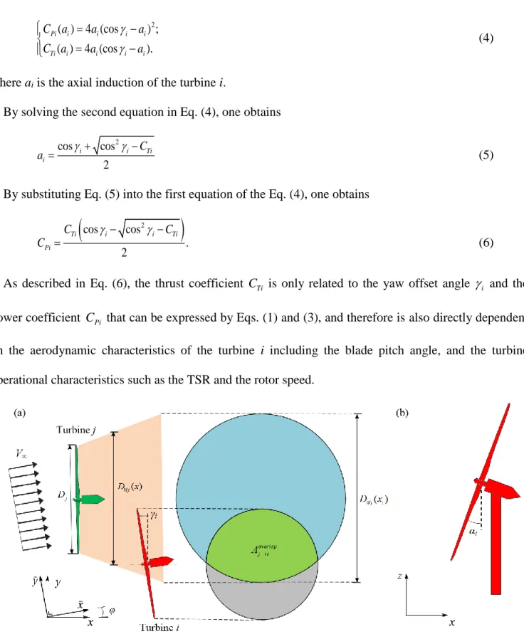
Fig. 1 The two turbine model example. (a) The wake expansion model of the turbines i and j (top view) (b) The tilt misalignment model of the turbine i (side view). In the Cartesian reference frame (x, y), the x

(10)

-Big data driven multi-objective predictions for offshore wind farm based on machine learning algorithms

9

axis points downwind along the free stream inflow direction, the y-axis is orthogonal to the x-axis along the crosswind direction, and the z-axis is orthogonal to the x and y axis, and represents the altitude. The reference frame ( , )x y is used to measure and represent the free stream inflow wind direction.

As shown in Fig. 1, the effective wind speed v t_i( ) seen by the turbine i in the wake of the turbine j is represented as [16]





( ) cos 1 ( )

i i

v t V_  v t (7)

where V_ is the free stream inflow wind speed, and φ is the angle of wind direction with respect to the x

axis, v t_i( ) is the fractional velocity deficit which can be given by [16]

 

2 , 2 ( ) 2 ; . 2 ( ) j i i j ji j F x x ol j ji ji j i j i v t a c D A c D k x x A     _           _ _ _ _ 



(8)

where k=0.084 denotes a tunable wake expansion coefficient, aj and Dj are respectively the axial induction factor and rotor diameter of the turbine j, Aol_ji denotes the overlapping area between the turbine i and the turbine j, xi and xj are respectively the x-axis coordinates of the turbine i and the turbine j.

As illustrated in Eqs. (1), (2), (7) and (8), the amount of total wind power production and thrust load of the turbine i is not only related to its own control inputs and the inflow wind parameters including the wind speed V_ and wind direction angle φ, but also is determined by the operational characteristics of the upstream turbine j due to the wake interactions. Therefore, under certain inflow wind speed and wind direction, the wind farm power and thrust outputs can be jointly determined by the control inputs of all the wind turbines in the wind farm, and the averaged wind farm power and thrust can be represented as

(11)

Big data driven multi-objective predictions for offshore wind farm based on machine learning algorithms 10 1 1 1 1 N F Wi i N F Wi i P P N T T N    _     



(9)

where P_F and T_F are respectively the averaged wind farm power output and the averaged wind farm

thrust.

2.2. Formulation of the wind farm prediction problem

As illustrated in the section 2.1, the wind farm power and thrust outputs are directly dependent on the control inputs of all the wind turbines, the turbine operational parameters, the inflow wind speed and direction. Therefore, by representing the input parameters of the offshore wind farm as a tuple, it is possible to construct a wind farm model as follows

 





; , ; ( , , , , , ). F F P T V_          y f x y x α β γ λ (10)

where f(V_, , , , , ) α β γ λ R2 is a vector-valued function representing the mapping from the tuple of admissible parameter settings to the averaged wind farm power and thrust,

, , N, N, N, N

V_R R αR βR γR λR are input vectors.

However, by observing Eqs. (1)-(10) in section 2.1, it is generally difficult to explicitly derive an analytical expression for Eq. (10) due to the core modeling challenges associated with the overlapping turbine wake interactions which increases levels of turbulence and shear and hence the complex dynamic loads of the downstream wind turbines. The wake interactions in a wind farm will become significant with the increasing number of wind turbines, thereby lowering the power productions and the reliability of the overall wind farm. In addition, the amount of the wake interactions depends on the operating point of each wind turbine, which is rather difficult to parametrize for a large wind farm. Therefore, rather than deriving

(12)

11

a detailed analytical wind farm model with wake interactions, the wind farm can be readily represented by training a machine learning model based on big sample data of input parameters V_, , , , α β γ and λ. This model is inherently multi-objective since the averaged wind farm thrust T_F is also used to represent the fatigue loads of the wind farm.

More specifically, the wake travelling dynamics will induce a delay in the model and hence the model needs to be extended with a delay time τ to consider the effects of the changes of input control variables on the entire wind farm outputs. Alternatively, the model can be employed to predict future farm responses based on the currently available control inputs. As a consequence, the machine learning model for Eq. (10) can be represented as y(t ) f



V t_( ), ( ), ( ), ( ), ( ), ( ) t α t β t γ t λt



, in which the tuple of the input parameters



V t( ), ( ), ( ), ( ), ( ), ( ) t α t β t γ t λ t



are specified as the predictor variables while the response variables can be specified as the future averaged values of P t_F( ) and T t_F( 



) since the number of turbines in a wind farm is a unique constant for the specific wind farm.

3. The data driven prediction methodology

The data driven machine learning approaches rely on sufficient data of the predictor and response variables while certain hyper parameters are optimized by minimizing pre-defined cost functions to attain the desired accuracy during iterations. For building machine learning systems that are stable, progressive and reliable for applications in offshore wind farm, five approaches are selected including the GRNN, the RF, the SVM, the GBR and the RNN. These approaches include both the standard machine learning methods such as the RF, SVM and GBR, and the deep learning architectures including the GRNN and RNN. The deep neural nets involve the high hierarchical architecture of many hidden layers and conduct the essentially multi-level non-linear operations through end to end optimizations [17]. Unlike the standard machine learning approaches, the deep neural nets also have distinctive attributes of the high-level more abstracted representation in learning the more complicated inherent structures.

(13)

12 3.1. The GRNN

The GRNN is built on the kernel regression, Bayes decision and nonparametric techniques for predicting the joint probability density function between inputs and outputs [18]. In the GRNN, the probability density function is assumed as the form of Gaussian distribution and thus no iterative training procedures are needed as in standard neural networks. The GRNN features high approximation accuracy, fast training speed and does not have local minima problem [19].

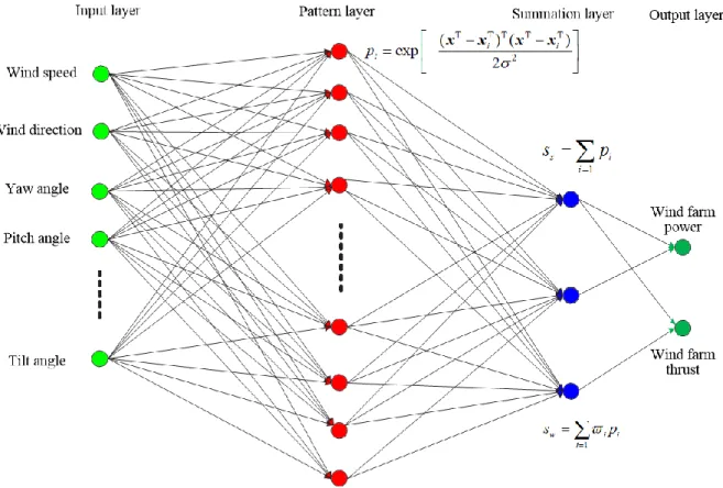
As illustrated in Fig. 2, the GRNN for predicting wind farm outputs are formulated into four layers: input layer, pattern layer (hidden layer), summation layer, and output layer. The input layer receives the input signals including wind speed, yaw angles, etc. In the pattern layer, neurons Gaussian functions to generate outputs from the input layer are as follows [18]

T T T T T 2 ( ) ( ) exp 2 i i i p       _ _   x x x x (11)

(14)

13

Fig. 2. The schematic diagram of the GRNN architecture

The summation layer has two types of summations: simple summation s_s and weighted summation s_w , each calculates the summations from the pattern layer as follows [19]

1 1 s i i w i i i s p s  p         



(12)

where



_i denotes the connecting weight between the pattern layer and summation layer.

The output layer has two neurons, each corresponding to the wind farm power and thrust. By feeding the outputs from the summation layer into the output layer, it is possible to calculate the GRNN output as [19] s w s y s  (13)

(15)

14 3.2. The RF

The RF is an extended and improved bagging method based on classification and regression trees and is also a non-parametric classification/regression approach [20]. In the RF, the training data are divided into an ensemble of multiple independent binary decision trees by using recursive partitioning and each tree is trained independently using different bootstrap samples on a random subset of the training data. For the construction of each regression tree, the RF randomly selects a random subset of variables at each node and thus this randomness process allows each tree to grow independently to its maximum size with continuous selection of the input variables at each node. Therefore, each tree acts as a regression function on its own and its accuracy can be tested based on the out-of-bag error of estimate which evaluates the relative importance of different evidential features. Approximately 30% of the new training sample constitutes the out-of-bag sample while two third sample is utilized for deriving the regression function.

The final predictions of RF are taken as the average of the responses from all the individual trees. The RF parameters include the number of independent variables that are randomly selected in each node and the maximum number of trees. Unlike neural networks, the RF is particularly robust and effective in modelling multi-source datasets with high dimensionality. The RF also provides an assessment of realistic prediction error estimates during the training process due to the built-in cross validation capability by using out-of-bag samples, which significantly improve its generalization capability. Another prominent advantage is that the trees of a RF grow with no pruning, which leads to much lighter computational burden and makes the RF suitable for real time implementation.

The implementation procedure of RF for predicting wind farm outputs can be designed as follows. (1). Determine the essential RF tuning parameters such as the number of trees and the maximum iterations.

(16)

15

(2). Randomly select a bootstrap sample with replacement from the available dataset and evolve each tree using bootstrapped sample taken from the dataset. Each tree is evolved to the maximum size without further splits and pruned back.

(3). Repeat step 2 until all the user-defined number of trees are grown.

(4). Evaluate the prediction error of the grown regression trees based on out of bag sample and calculate the averaged error.

(5). Obtain the tree outputs for the given inputs such as pitch angles and yaw angles and obtain the final predictions including the wind farm power and thrust by averaging the predictions of all the trees.

3.3. The SVM

The SVM is a popular nonparametric machine learning tool relying on kernel functions and has great generalization ability in dealing with complex systems and corrupted data [21]. Unlike the empirical risk minimization principle used in neural networks, the structural risk minimization is used in the SVM to find the best regression hyperplane in a “high dimensional feature space”. Therefore, the basic principle is to map the low-dimensional space data input into a high dimensional feature space by constructing a separating hyperplane with the maximum margin in the feature space [22]. This nonlinear transformation is accomplished by using Kernel functions that satisfy the Mercer’s condition [23].

Given a set of sample data (xi, yi), i = 1, 2, ..., n, where n is the quantity of the sample data, the approximate linear mapping from the input to output can be formulated based on SVM as follows [21]

T

ˆ( ) ( )

y k ω  x b (14)

where y kˆ( ) is the estimated outputs for wind farm power and thrust, k=1, 2,



( )x is a nonlinear mapping from the input to the output, ωRm and bR are respectively the weights and a bias constant, m is the number of features.

(17)

Big data driven multi-objective predictions for offshore wind farm based on machine learning algorithms 16 *T ( ) ( ) ˆ ( ) ( ) y k b y k y k        _ _  ω x (15)

where ε > 0 is a arbitrarily small positive constant, _ω*_ m

R is the optimal value of ω.

Then, the prediction problem can be transformed into the following optimization problem [22].

T 2 1 T 1 1 min 2 2 s.t. ( ) ( ) n k i i i m C y k b        



ω ω ω x (16)

where C and



_i are respectively a positive box constraint and a positive slack variable, m_k is a weight coefficient.

By using Lagrangian multiplier



_iR, the above optimization problem in Eq. (16) can be described as [23] T 2 T 2 1 1 1 1 ( ) ( ) 2 2 n n k i i i i i i i L m C    b  y k       ω ω

 

 _ω x    _ (17) In order to solve Eq. (17) analytically, the following equations should be satisfied

1 T 1 ( ); ; 0; 0; 0; 0. _0; _{( )} _{( ) 0.} n i i i k i i n i i i i i i L L m C b L L b y k                _ _ _ _     _ _ _   _ _  _ _{  } _      



ω x ω ω x (18)

The solution to Eq. (18) yields T 1 ( ) ( ) ( ) n i i i j i i k b y k m C        



x x (19)

The above solution in Eq. (19) can also be expressed as follows [24] T , -1 T ( ) ( ) ( , ); 0 ; ( ) i j i j K i j b y k                      Q x x x x Q φ (20)

(18)

17 where K x x( ,_i _j) is a kernel function.

1 1 1 1 1 1 0 1 ... 1 1 ( , ) ( ) ... ( , ) ... ... ... 1 ( , ) ... ( , ) ( ) k n n n n k K m C K K K m C      _        _    x x x x φ x x x x (21)

Based on Eqs. (20) and (21), the prediction from the SVM can be formulated as

1 ( ) ( , ) n i i j i y k K b  



x x  (22)

In order to improve the prediction performance, different custom Kernel functions can be specified such as the radial basis function or hybrid kernel function that meet the Mercer’s condition [24]. According to the above descriptions, the SVM essentially locates the hyperplane with a ε-insensitive loss function in Eq. (15) and thus tolerates errors that are within ε distance of the predicted values. The SVM is also memory efficient due to the use of support vectors in the decision function and is thus still effective in dealing with the cases where the number of features is greater than the number of samples. Therefore, the SVM is particularly suitable for predicting the large scale wind farms outputs.

3.4. The GBR

The GBR is a relatively new prediction approach for representing high order feature interactions based on the combination of both machine learning and statistical boosting. The GBR is characterized by regression trees and boosting and can produce a prediction model in the form of an ensemble of decision trees [25], [26]. A large ensemble of regression trees are grown like a form of recursive partitioning by randomly selecting a certain amount of training data without replacement. Recursive splits are employed in the regression trees to subdivide the predictor space into non-overlapping regions, thereby identifying regions with most homogeneous responses to predictors. Unlike the conventional bagging in the RF, the special mechanism “boosting” applied in GBR can effectively reduce the variance in bootstrapping

(19)

18

samples and thus can form a low-variance predictor. In boosting, an ensemble of simple base learners are built and combined in a repeatedly iterative stage-wise process, resulting in distributions that concentrate on more difficult training cases. In order to prevent overfitting, the small trees, each with high bias are sequentially added and averaged in the GBR. Therefore, the regression trees are robust to outliers in the data and are insensitive to the inclusion of irrelevant variables [27].

In order to evaluate the prediction results, a loss function is typically specified, such as a mean squared-error loss function, and gradient boosting is used to learn these boosted regression trees based on a learning rate. The main tuning parameters of the GBR for optimizing predictive accuracy include the proportion of data that are drawn without replacement at each iteration, and the number of trees [28].

By introducing the boosting technique, the stability and accuracy of the GBR can be highly improved, giving rise to a single very strong predictive model. As compared to other methods, the GBR with hierarchical structure holds several prominent advantages including high invariance under transformations of the predictors, high tolerance to outliers, and the capability to handle missing data and include both continuous and categorical variables [29]. In addition, the GBR also lends itself to the recovery of the informational content of leading predicators by capturing even complex regression nonlinearities in a natural way.

3.5. The RNN

Unlike standard feedforward neural networks, the RNN has feedback connections or a “recurrent” structure and performs the current prediction using not only the input data, but also the previous outputs. The gradient backpropagation through time (BPTT) algorithm is implemented in the model training of RNN to compute the gradient descent after each iteration [30]. However, during the BPTT of many time steps, the RNN suffers from the problem of vanishing or exploding gradients whose values become extremely small or large. In order to tackle this issue, the popular long-short term memory (LSTM) cells

(20)

19

can be used for deep RNN in learning long-term dependencies. The LSTM cell is a specifically designed gated memory unit of logic with internal mechanisms called gates that can regulate the flow of information.

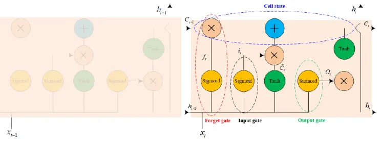
As shown in Fig. 3, a typical LSTM cell consists of three gates that manage the contents of the memory, the input gate, the output gate and the forget gate. The three gates are simple logistic functions of weighted sums, where the weights are trained by using the BPTT method. The input gate and the forget gate manage the long-term memory cell state. The output gate generates the output vector or hidden state, which is the memory focused for use. The forget gate is used to control the time dependence and effects of previous inputs and can determine which states are remembered or forgotten.

Considering the representation of two repeating LSTM cells for a RNN as pictured in Fig. 3, the time or sequence-dependent data flow from left-to-right, with the current input xt and the previous cell output

ht−1 concatenated together and entering the right “data rail”.

Fig. 3 The architecture of two repeating LSTM cells containing four interacting layers

As shown in Fig. 3, the forget gate decides what is relevant to keep from prior steps by passing the information of the current input xt and the previous cell output ht−1 through the sigmoid function. Therefore, the current hidden output is updated as follows [31].







1



sigmoid ,

t f t t f

(21)

20

where ft is the output from the forget gate, the square bracket [ , ] denotes the vector concatenation, Wf and

bf denote the weight and bias vectors for the forget gate, respectively.

The input gate decides what information is relevant to add from the current input xt and the previous cell output ht−1. The current internal state is then updated from the outputs from the input gate and forget gate [31]. Hence,

















1 1 1 sigmoid , ; tanh , ; . t i t t i t c t t c t t t t t i W h x b C W h x b C f C i C         _ _ _        (24)

where it is the output from the input gate, Ct, Ct-1 and Ct are internal state variables, Wi and Wc are respectively the weight vectors for the input gate and internal state, bi and bc are respectively the biases for the input gate and internal state, tanh() denotes the hyperbolic tangent function, and * denotes the pointwise multiplication.

The output gate determines what the next hidden state should be. In the output gate, the squashed state is multiplied by the output sigmoid gating function to determine which values of the state are output from the cell. The output gate takes the following form [31]







1



sigmoid , ; tanh( ). t o t t o t t t O W h x b h O C           (25)

Then, the next LSTM cell follows the similar procedure, and updates the cell state and output to new values as a function of the values of the hidden state and the output at the current time step and the value of the cell input at the next time step.

The above-mentioned sigmoid function squishes values between 0 and 1, and the tanh function squishes values between -1 and 1. Therefore,

(22)

Big data driven multi-objective predictions for offshore wind farm based on machine learning algorithms 21 exp( ) exp( ) tanh( ) ; exp( ) exp( ) exp( ) sigmoid( ) . exp( ) 1 x x x x x x x x    _  _ _    _    (26)

4. Case studies and validations

The assessment of the above-mentioned data driven machine learning approaches has been conducted based on a wind farm simulation platform named FLORIS that was developed by the National Renewable Energy Laboratory (NREL) and the Delft University of Technology [32]. The FLORIS model is a calibrated data-driven parametric tool for performing real-time optimizations to improve wind farm performance. This tool implements a 3D version of the Jensen and Gaussian wake model, and is designed to provide a computationally inexpensive and controls-oriented model of the steady-state wake characteristics in a wind farm. By combining the Jensen model [33], wind inflow properties (wind speed and direction), and a model for wake deflection through turbine yaw settings, the FLORIS is programmed using Python language to better model situations with wake deflection, partial wake overlap and wake position offsets caused by rotor rotational effects.

The turbine model employed in the FLORIS is the NREL 5 MW turbine and the wind farm comprised of 4 × 5 MW wind turbines was used for data acquisition [34]. The turbine model consists of power and thrust coefficients while the wind field modeling considers turbulences, wake effects, inflow wind speeds and directions. For the purpose of easy demonstration, the averaged power and thrust are measured as the wind farm outputs, and the turbine yaw angle settings are fed into the model as control inputs while other input parameters including the blade pitch angle, the tilt angle, and the turbine operational characteristics such as the TSR and the rotor speed are kept constant.

Hence, the corresponding farm power and thrust outputs in conjunction with those yaw angle settings are employed as the basis for training and testing the machine learning approaches presented in section 3. Different scenarios with different wind inflow properties are used to assess the prediction accuracy of the

(23)

22

machine learning approaches. All case studies were carried out using Python 3.6.8 on an Intel Core i7-7700 OptiPlex 7050 Dell desktop with 3.60 GHz 8 CPUs and 32, 768 MB RAM.

4.1. The prediction settings and data preprocessing

The sequences of input and output data of the wind farm were generated by using the FLORIS, consisting of a training and a validation dataset. The input yaw angle settings for the data generations in the FLORIS were randomly generated as a sample sequence consisting of four elements between -35° and 35°, and each yaw angle is fully distinguished from the previous yaw angle settings. The total number of yaw angle settings are respectively 360, 000 and 36, 000 for the training and validation datasets. Typical operating scenarios and patterns of the wind farm are extracted to facilitate the wind farm predictions. The scenarios include 6 different inflow wind speeds and directions: the mean wind speeds of 8 m/s, 16 m/s and 28 m/s with 270° wind direction, and the wind directions of 180°, 225° and 315° with 16 m/s inflow wind speed. All the scenarios are set with the turbulence intensity of 6% in order to evaluate the prediction performances of these approaches under both low and high turbulent wind conditions. Note that the wind directions in all the scenarios are set by following the FLORIS convention and maybe different from the angle of wind direction φ in Fig. 1.

The training and validation of the machine learning approaches based on the FLORIS data were conducted by using a number of fundamental Python packages such as the NumPy and the SciPy, and popular machine learning libraries including the Tensorflow, the Scikit-learn, the Theano, and the Keras. The NumPy library is used to perform high-level mathematical functions on multi-dimensional arrays and matrices [35], and the SciPy library is used for scientific computing and data processing [36]. The machine learning framework of Tensorflow is an open-source software library for deep learning neural networks and dataflow programming across a wide range of tasks [37]. The Scikit-learn library features various classification, regression and clustering algorithms including support vector machines [38]. The Theano

(24)

23

library features tight integration with NumPy, efficient symbolic differentiation, speed and stability optimizations and has been used for large-scale computationally intensive scientific investigations [39]. The Keras library is used for developing and evaluating deep learning models with either the Tensorflow or Theano backend [40]. By wrapping the efficient numerical computation libraries from the Theano and Tensorflow, the Keras is a powerful Python library for defining and training neural network models in a few short lines of codes.

The settings for the five machine learning approaches are listed as follows.

GRNN. The GRNN was constructed in Python by using the Tensorflow and the NumPy. The GRNN has a deep learning architecture with three hidden layers (or pattern layers as shown in Fig. 2). The numbers of neurons in the three hidden layers are set respectively as 512, 256 and 128. For fitting the GRNN, the batch size and epochs are set respectively as 100 and 50.

RF. The RF algorithm was constructed by using RandomForestRegressor imported from the

sklearn.ensemble in the Scikit-learn library. The maximum depth, the number of estimators and the random state are set as 30, 100 and 2, respectively for training the RF.

SVM. The SVM was constructed by using the SVR (support vector regression) imported from the

sklearn.svm in the Scikit-learn library. The used kernel is the radial basis function, and the parameters C,

gamma and epsilon in the trained SVR model are respectively set as 1×103, 0.9 and 1×10-3.

GBR. The GBR was constructed based on the ensemble model from the sklearn package. The number of estimators, the maximum depth, the minimum sample split and the learning rate are set as 500, 8, 2 and 0.01, respectively for fitting the GBR. The individual regression tree is grown by using the gradient boosting to minimize the least squares loss.

RNN. The RNN was defined and trained by using the Keras library. The RNN model defines the LSTM with 50 neurons in the first hidden layer and 2 neurons in the output layer for predicting the wind farm

(25)

24

power and thrust. The input shape is set as 1 time step with 4 features. The mean absolute error (MAE) loss function and the efficient adam optimizer of stochastic gradient descent were used for training the LSTM RNN model. The RNN model has been fit for 100 training epochs with a batch size of 60.

The following commonly used comparison metrics in Eqs. (27)~(30) are used to assess the accuracy of the machine learning approaches since they have been extensively used to describe the data prediction accuracy.

The relative percentage error (RPE):

ˆ RPE i i 100% i y y y    (27) where yi and ˆy_i are respectively the real value and the prediction value, i is the index of the predictions.

The mean absolute percentage error (MAPE)

1 ˆ 1 MAPE 100% n i i i i y y n  y  



 (28) The minimum absolute relative percentage error (MARPE)

ˆ MARPE min i i 100% i y y y  _   __  __   ₍₂₉₎

The root mean square error (RMSE)





2 1 1 _ˆ RMSE n i i i y y n  



 (30) As illustrated in the above Eqs. (27)~(30), the relative errors are calculated by dividing the errors between the real and predicted values by the corresponding real values, while the absolute errors are calculated by taking the absolute values of these relative errors. In addition, the CPU time for implementing the algorithms is also employed as an important metric for evaluating the computational

(26)

25

efficiency of the five algorithms. For each scenario, the algorithms are ranked by 1 to 5, where 1 represents the best and 5 represents the worst.

4.2. The prediction results under different wind speeds

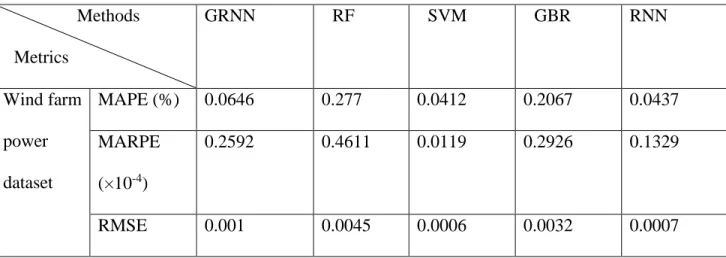
This section presents the prediction results under different inflow wind speeds of 8 m/s, 16 m/s and 28 m/s while the wind inflow direction is fixed at 270°. The prediction results under 8 m/s wind speed are presented in Table. 1 and Figs. 4 and 5. In this scenario, the validation data has 6000 samples and the prediction results are extremely accurate. As illustrated in Table. 1, the SVM has the best performance in wind farm power prediction, while the RNN has the best performance in predicting wind farm thrust. The minimum MAPE (%) for wind power prediction is 0.0412 % and the minimum MAPE (%) for wind farm thrust prediction is 0.0258%, which indicate that the relative accuracies (calculated by (100%-MAPE)) of wind farm power and thrust predictions can achieve 99.9588% and 99.9742%, respectively. Although the five algorithms have been ranked from 1 to 5, there exist very minor differences among them. The lowest relative prediction accuracy can still achieve 99.7%, which is sufficient for data-driven wind farm predictions. The GRNN uses only 0.037s to process 6000 data samples, which means each data sample can be processed in 5µs by using the GRNN. Therefore, it is clear that the GRNN has the best computational efficiency.

Table 1. The prediction results under 8 m/s free stream wind speed Methods Metrics GRNN RF SVM GBR RNN Wind farm power dataset MAPE (%) 0.0646 0.277 0.0412 0.2067 0.0437 MARPE (×10-4) 0.2592 0.4611 0.0119 0.2926 0.1329 RMSE 0.001 0.0045 0.0006 0.0032 0.0007

(27)

Big data driven multi-objective predictions for offshore wind farm based on machine learning algorithms 26 CPU time (s) 0.0369 0.1676 0.365 0.1666 0.1486 Rank 3 5 1 4 2 Wind farm thrust dataset MAPE (%) 0.066 0.2223 0.069 0.191 0.0258 MARPE (×10-4) 0.2119 0.0415 0.0843 0.0024 0.1234 RMSE (×10-3) 0.2305 0.9079 0.2380 0.7158 0.0893 CPU time 0.0379 0.1496 0.1666 0.1468 0.2126 Rank 2 5 3 4 1

As shown in Fig. 4, the predicted averaged wind farm power and thrust coincide highly with the real values. It is really difficult to distinguish the differences between the prediction results from the RNN and SVM, while the prediction results from the GRNN, RF and GBR can be observed clearly. The prediction results indicate that the RNN and SVM have the best prediction accuracy which is in good agreement with the results as shown in Table. 1.

(28)

27

Fig. 4. The wind farm prediction results under 8 m/s free stream wind speed (a) Wind farm power (b) Wind farm thrust

(29)

28

As shown in Fig. 5(a), the RNN and SVM have the best RPE values which are clearly between ±0.3%, while the RF and GBR have much higher RPE values between -2.5% and 1.5%. As shown in Fig. 5(b), the RNN clearly has the lowest RPE values and the RPE values of the RF and GBR are much higher. Therefore, the RNN and SVM have the best prediction accuracy and the RNN exhibits the best accuracy in wind farm thrust predictions.

(30)

29

Fig. 5. The RPE results under 8 m/s free stream wind speed (a) Wind farm power dataset (b) Wind farm thrust dataset

Table. 2 and Fig. 3 illustrate the results for the 6000 data points of power and thrust predictions by using the five algorithms under the inflow wind speed of 16 m/s. For the wind farm power prediction, the SVM has the best accuracy with the MAPE of only 0.0118% and the RF performs the worst. For the wind farm thrust prediction, the RNN holds the best accuracy while the RF performs the worst. In terms of the CPU time, the GRNN prediction is the best (around 0.04s for 6000 data points). However, the differences among the five algorithms are very minor, and all of them can achieve the relative prediction accuracy of 99% which is enough for wind farm prediction applications.

Table 2. Prediction results under 16 m/s free stream wind speed Methods

Metrics

(31)

Big data driven multi-objective predictions for offshore wind farm based on machine learning algorithms 30 Wind farm power dataset MAPE (%) 0.0827 0.4209 0.0118 0.3091 0.0403 MARPE (×10-4) 0.0557 0.5342 0.0624 02029 0.1005 RMSE 0.0049 0.0264 0.0007 0.019 0.0023 CPU time (s) 0.0329 0.1766 0.362 0.1596 0.1275 Rank 3 5 1 4 2 Wind farm thrust dataset MAPE (%) 0.1822 0.4319 0.0755 0.317 0.041 MARPE (×10-3) 0.0085 0.1813 0.053 0.0061 0.0104 RMSE 0.0008 0.0021 0.0003 0.0015 0.0002 CPU time (s) 0.0419 0.1626 0.1686 0.1576 0.2099 Rank 3 5 2 4 1

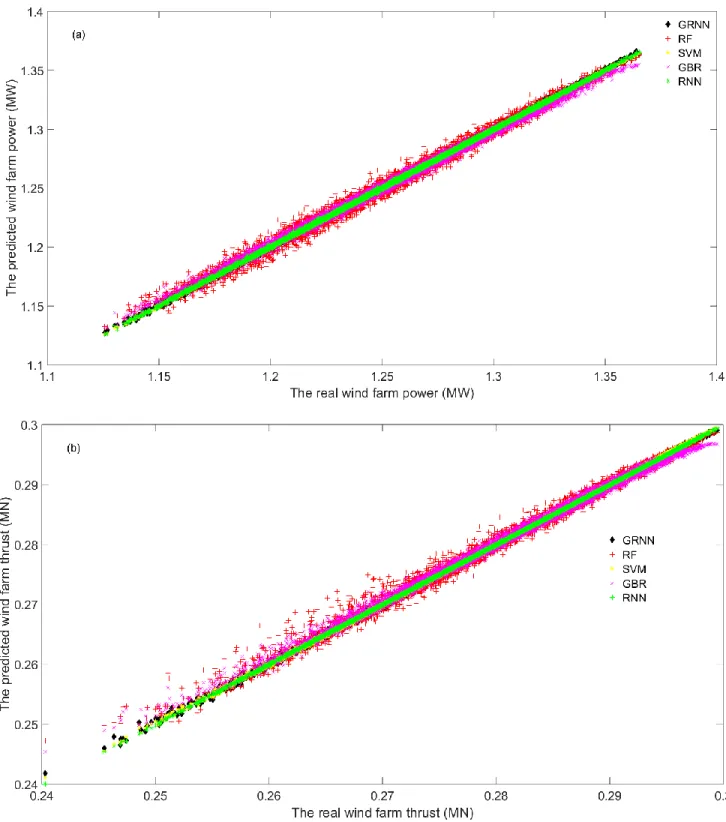
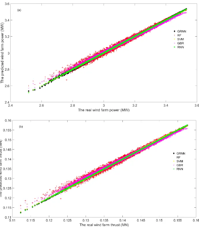
As shown in Fig. 6, the RNN and SVM can almost achieve the same and best prediction performances in wind farm power and thrust predictions since their prediction points are almost located at the accurate positions of the accurate 45° diagonal straight line across the figure and it is rather difficult to distinguish them. The prediction points from the RF and GBR clearly distribute more widely around the accurate points and hence their prediction accuracies are a little lower.

(32)

31

(33)

32

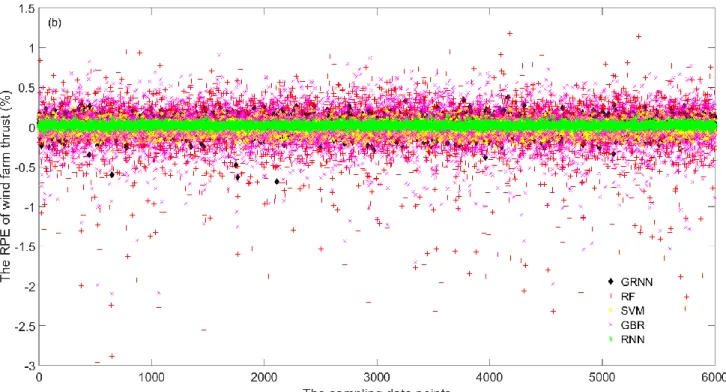
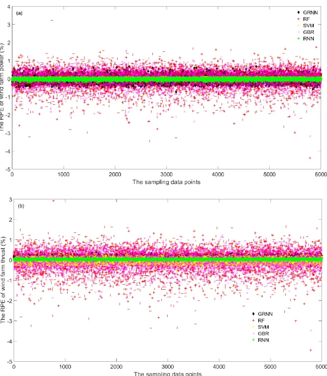
As shown in Fig. 7(a), the RNN and SVM clearly exhibits the best RPEs in comparison with the other three algorithms. The RNN has the lowest RPE values than the other four algorithms as shown in Fig. 7(b). The prediction results by using GBR and RF are distributed sporadically between -5% and 2%. The RNN and SVM clearly have the best prediction accuracy and particularly the wind farm thrust prediction accuracy of the RNN is the best. The results of the RPE values also have good agreement with those presented in Table. 2.

(34)

33

The prediction results of the wind farm under 28 m/s inflow wind speed are presented in Table. 3, Figs. 8 and 9. As illustrated in Table. 3, the RNN is ranked the best in wind farm power and thrust predictions while the SVM is ranked the second. The minimum MAPE is 0.0437% for power prediction while the minimum MAPE is about 0.0377% for thrust prediction. The minimum CPU time has been achieved by using the GRNN and the time for processing 6000 data samples can be made as low as 0.0329s. The differences of the prediction performances in the five algorithms are really minor and the RF can still achieve the relative good accuracy of 99.58%, which is the lowest, but is enough for wind farm prediction applications.

Table 3. Prediction results under 28 m/s free stream wind speed Methods

Metrics

(35)

Big data driven multi-objective predictions for offshore wind farm based on machine learning algorithms 34 Wind farm power dataset MAPE (%) 0.1432 0.4153 0.053 0.3063 0.0437 MARPE (×10 -3₎ 0.0165 0.1328 0.0096 0.124 0.019 RMSE 0.0055 0.017 0.0019 0.0124 0.0018 CPU time (s) 0.0329 0.1731 0.1805 0.1581 0.1207 Rank 3 5 2 4 1 Wind farm thrust dataset MAPE 0.1236 0.4202 0.1071 0.3094 0.0377 MARPE (×10 -3₎ 0.1563 0.0117 0.001 0.0177 0.0283 RMSE (×10-3) 0.194 0.7676 0.1798 0.5588 0.0613 CPU time (s) 0.0489 0.1371 0.0459 0.1694 0.1297 Rank 3 5 2 4 1

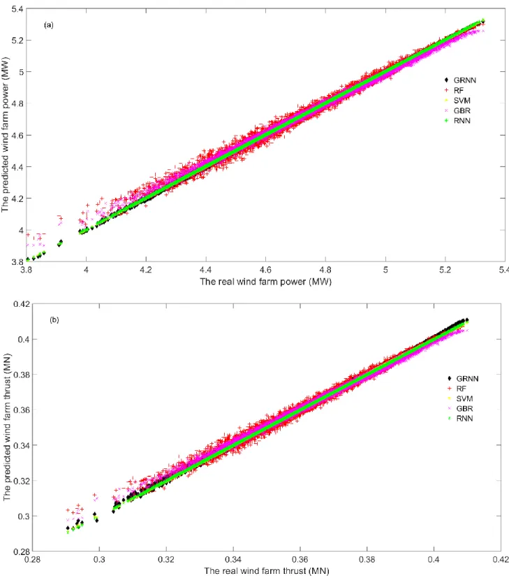
As shown in Fig. 8, the prediction points from the RNN and SVM are in very good agreement with their real values while the points predicted by the GRNN have a little bit deviations from the real values. The prediction points from the RF and GBR are located much widely around the accurate 45° diagonal straight line across the figure, which means their prediction performances are not as good as the RNN and SVM.

(36)

35

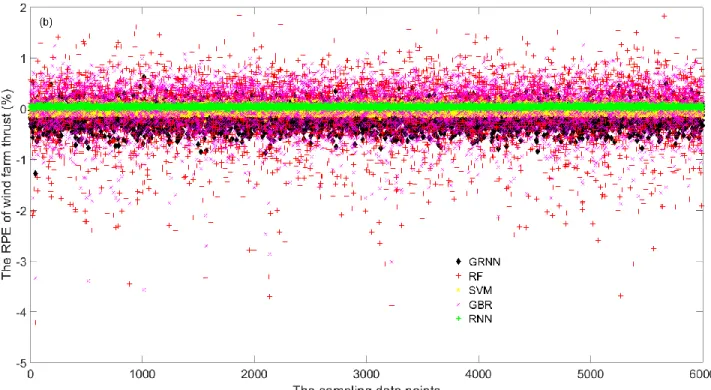
As shown in Fig. 9(a), the RPE values of the RNN and the SVM are most converged around 0, while the RPE values of the GRNN, the RF and the GBR varies between -5% and 3%. As shown in Fig. 9(b),

(37)

36

the RNN has the most converged and lowest RPE values around 0 in comparison with the other four algorithms. It is clear that the RNN and SVM have the narrowest range of RPE, and particularly the RNN has the best performance in wind farm thrust predictions.

(38)

37 4.3. The predication results under different wind directions

This section presents the prediction results under different inflow wind directions of 180°, 225° and 315° with constant inflow wind speed of 16 m/s.

Table. 4 and Figs. 10 and 11 show the prediction performance comparisons of the five algorithms with 6000 sample data points under 180° wind direction. The SVM outperforms others in power predictions while the RNN outperforms others in thrust predictions, and the corresponding values of MAPE are respectively 0.0247% and 0.0363%. The GRNN has the lowest computation time (0.03s for processing 6000 data samples) in the two cases and hence is the most computationally efficient. The differences among these algorithms are really minor – each of them can achieve a prediction accuracy of at least around 99%.

Table 4. Prediction results under 180° wind direction Methods Metrics GRNN RF SVM GBR RNN Wind farm power dataset MAPE (%) 0.1795 0.4178 0.0247 0.3074 0.0357 MARPE (×10-4₎ 0.1688 0.6140 0.0014 0.0235 0.2043 RMSE 0.0098 0.0258 0.0014 0.0187 0.0021 CPU time (s) 0.0309 0.1775 0.0698 0.1605 0.2262 Rank 3 5 1 4 2 Wind farm MAPE (%) 0.063 0.4641 0.0537 0.3427 0.0363 MARPE (×10-4) 0.3112 0.9986 0.065 0.0426 0.1002

(39)

Big data driven multi-objective predictions for offshore wind farm based on machine learning algorithms 38 thrust dataset RMSE 0.0003 0.0023 0.0002 0.0016 0.0002 CPU time (s) 0.0329 0.1646 0.1396 0.1616 0.1287 Rank 3 5 2 4 1

The comparisons between the real values and the predicted values from the five algorithms are shown in Fig. 10. As illustrated in this figure, the RNN and the SVM have the best prediction performances since their prediction points are almost aligned with the 45° diagonal straight line across the figure. The predicted data points from the other three algorithms have a little deviations from the 45° diagonal straight line, which means their prediction performances are not as good as the RNN and the SVM.

(40)

39

Fig. 10. The wind farm prediction results under 16 m/s wind speed and 180° wind direction (a) Wind farm power (b) Wind farm thrust

The similar prediction results can be found in Fig. 11 as those in Table. 4 and Fig. 10. The RPEs of RF and GBR scatter widely between -5% and 3% while the RPEs of RNN and SVM can be well bounded between ±0.05%, which are clearly smaller than those of the GRNN and GBR. The discrepancies revealed in Fig. 11 for the five methods are in good agreement with that in Table. 4 and Fig. 10, which suggests that the RNN and SVM are the best choices for wind farm power prediction while the RNN is the best choice for wind farm thrust prediction.

(41)

40

Fig. 11. The RPE results under 16 m/s wind speed and 180° wind direction (a) Wind farm power dataset (b) Wind farm thrust dataset

The prediction performance and test results of the wind farm under 225° by using 6000 sampling data points are presented in Table. 5, Figs. 12 and 13. As shown in Table. 5, the SVM performs the best in

(42)

41

wind farm power prediction while the RNN has the best accuracy in predicting wind farm thrust. The corresponding MAPEs are respectively 0.0318% and 0.0303%. The GRNN outperforms the SVM in wind farm thrust prediction, and it only needs 0.0309s CPU time for processing 6000 data points. The prediction performances of all the five algorithms are also in good agreement with the previous cases and 99% relative accuracy can be readily reached by all the five methods, which suggests that these methods can be readily used in wind farm predictions.

Table 5. The prediction results under 225° wind direction Methods Metrics GRNN RF SVM GBR RNN Wind farm power dataset MAPE (%) 0.0978 0.4314 0.0318 0.3061 0.0322 MARPE (×10-4) 0.0653 0.0092 0.0613 0.1882 0.1117 RMSE 0.0058 0.0272 0.0018 0.0189 0.0018 CPU time (s) 0.0319 0.1775 0.1835 0.1642 0.2439 Rank 3 5 1 4 2 Wind farm thrust dataset MAPE (%) 0.0439 0.4325 0.0821 0.3116 0.0303 MARPE (×10-4) 0.2963 0.7803 0.021 0.2985 0.1152 RMSE 0.0002 0.002 0.0003 0.0014 0.0001 CPU time (s) 0.0309 0.1596 0.1556 0.1631 0.1231 Rank 2 5 3 4 1

(43)

42

As illustrated in Fig. 12, the prediction points from the RNN and the SVM are almost aligned with the accurate the 45° diagonal straight line and it is very difficult to distinguish them, which means the RNN and the SVM have the best prediction performances. On the other hand, the prediction points from the GBR and the RF scatter much widely in the figure, which suggest their performances are not as good as the RNN and the SVM.

(44)

43

As illustrated in Fig. 13, both the RNN and SVM achieve much bounded RPEs within ±0.05%, whereas the RPEs of the RF and GBR varies more widely 2% and -6%. More particularly, the RPE of the RNN is obviously smaller than that from the SVM as shown in Fig. 13(b) which means the RNN outperforms the SVM in wind farm thrust predictions. All the RPE results also agree very well with those in Table. 5 and Fig. 12.

(45)

44

Fig. 13. The RPE results under 225° wind direction (a) Wind farm power dataset (b) Wind farm thrust dataset

(46)

45

The prediction performances of the five algorithms under 225° wind direction and 16 m/s inflow wind speed are compared in Table. 6, Figs. 14 and 15. The results indicate similar discrepancies between the wind farm power and thrust predictions as those in the aforementioned cases. The prediction model derived by the SVM outperforms other models in predicting the wind farm power while the RNN has the best performances in predicting the wind farm thrust. The GRNN model is the most computationally efficient and has relatively high prediction accuracy. All the five methods have very minor differences in wind farm predictions and the relative prediction accuracy can reach 99%.

Table 6. The prediction results under 315° wind direction Methods Metrics GRNN RF SVM GBR RNN Wind farm power dataset MAPE (%) 0.0854 0.4129 0.0314 0.3001 0.0369 MARPE (×10-3) 0.0156 0.0318 0.044 0.1089 0.0016 RMSE 0.005 0.0258 0.0017 0.0185 0.0022 CPU time (s) 0.0339 0.1785 0.1655 0.1636 0.1326 Rank 3 5 1 4 2 Wind farm thrust dataset MAPE (%) 0.0930 0.4199 0.0765 0.3054 0.0451 MARPE (×10-4) 0.7858 0.298 0.0829 0.1652 0.067 RMSE 0.0005 0.002 0.0003 0.0014 0.0002 CPU time (%) 0.0319 0.1676 0.1476 0.1636 0.1337

(47)

46

Rank 3 5 2 4 1

As obviously shown in Fig. 14, almost all the prediction points from the RNN and the SVM are located around the accurate 45° diagonal straight line and it is very difficult to distinguish them. The prediction points from the GRNN have a little deviations from the accurate 45° diagonal straight line while the prediction points from the GBR and the RF scatter much widely around the accurate 45° diagonal straight line. All the results reveal that the RNN and the SVM have the best prediction performances while the GRNN can be ranked as the third.

(48)

47

As obviously shown in Fig. 15, the differences of the RPEs of the five methods can be discerned in wind farm power and thrust predictions. The convergence ranges of the RF and SVM can be achieved between ±0.05%, while the RPEs of the GRRN and GBR vary widely between 2% and -5%, which shows good agreement with the aforementioned results and indicates the RNN and the SVM have the best prediction accuracy.

(49)

48

Fig. 15. The RPE results under 16 m/s wind speed and 315° wind direction (a) Wind farm power dataset (b) Wind farm thrust dataset

By comparing the prediction results in sections 4.2 and 4.3, very good agreement can be achieved among the five typical machine learning methods during the 6 different scenarios. The RNN and the SVM

(50)

49

exhibit the best prediction accuracy, and particularly the RNN has the best accuracy in wind farm thrust predictions. The GRNN uses the lowest CPU time for processing dataset and is the most computationally efficient. The differences among the five methods are rather minor and all the five algorithms hold very high prediction accuracy of around 99%, which are suitable for wind farm predictions. In addition, the five typical machine learning methods for prediction purpose can also be applied in other typical energy systems including the vibrational energy harvesters [41]~[43].

5. Conclusion

This paper has investigated the big data-driven multi-objective prediction framework for predicting the wind farm power output and structural fatigue. The prediction framework was synthesized by using the averaged wind farm power output and the equivalent thrust of turbine as the response variables and the wind conditions, control settings and turbine characteristics as predictor variables. The prediction models were subsequently constructed with five different data mining algorithms including the GRNN, the RF, the SVM, the GBR, and the RNN. The prediction performances of the five approaches were compared and evaluated based on the most recent version of FLORIS. The test results have validated that all these methods can achieve the relative accuracy of around 99% or more, which is good enough for practical applications. The RNN and SVM exhibit the best accuracy, and particularly the RNN has the best accuracy in thrust predictions. The results also demonstrate that the GRNN has the best computational efficiency.

Acknowledgement

This work is supported by the UK Engineering and Physical Sciences Research Council (grant number: EP/R007470/1).

References

[1] World Energy Resources: Wind 2016. https:.www.worldenergy.org/wp-content/uploads/2017/03/WEResources_Wind_2016.pdf.