FAST ACTIVE QUEUE MANAGEMENT SCALABLE TRANSMISSION CONTROL PROTOCOL, A NEW TCP VARIANT, AN EFFICIENT TCP

320 | P a g e

FAST ACTIVE QUEUE MANAGEMENT SCALABLE

TRANSMISSION CONTROL PROTOCOL, A NEW

TCP VARIANT, AN EFFICIENT TCP

Sudhir A. Shinde

, Dr. Dinesh. B. Kulkarni

Student of M.E. (CSE), Walchand College of Engineering, Sangli (India)

Professor and Head in IT Department, Walchand College of Engineering, Sangli(India)

ABSTRACT

Fast Active Queue Management Scalable Transmission Control Protocol, a new TCP congestion control algorithm is designed and implemented for high-speed long-latency networksis described in this paper. The current TCP implementation addresses the four difficulties at large windows. The approach is taken by FAST TCP to address these four difficulties.The architecture and summaryof some of the algorithms implemented. Its equilibrium and stability properties are also characterized. The experimental setup in terms of throughput, fairness, stability, and responsiveness is evaluated.

Keywords - FAST TCP, Implementation, Internet Congestion control, Protocol Design, Stability Analysis.

I. INTRODUCTION

Congestion control is a distributed algorithm to share network resources. It is important in the situations where

the availability of resources and the set of competing users vary over time unpredictably. These constraints,

unpredictable supply, demand and efficient operation, leads to feedback control. The approach, where traffic

sources dynamically adapt their rates to congestion in their paths. On the internet this is performed by the

Transmission Control Protocol (TCP) in source and destination computers involved in data transfers.

The congestion control algorithm in the current TCP, which is referred as Reno in this paper, was developed in

1988.And it has gone through several enhancements. It has performed remarkably well.This is generally

believed to have prevented severe congestion as the internet scaled up by six orders of magnitude in size, speed,

load and connectivity. The following four difficulties will contribute to the poor performance of TCP Reno in

networks with large bandwidth and delay products.

1. At the packet level, linear increase by one packet per round- trip time (RTT) is too slow, and multiplicative

decrease per loss event is too drastic.

2. At the flow level, maintaining large average congestion windows requires an extremely small equilibrium loss

probability.

3. At the packet level, oscillation in congestion window is unavoidable because TCP uses a binary congestion

signal (packet loss).

4. At the flow level, the dynamics is unstable, leading to severe oscillations that can only be reduced by the

accurate estimation of packet loss probability and a stable design of the flow dynamics.

II. PROBLEMS AT LARGE WINDOWS

A congestion control algorithm can be designed at two levels. The macroscopic flow-level design aims to

321 | P a g e

implements these flow level goals within the constraints imposed by end-to-end control [2].

2.1 Packet and flow level modelling

The congestion avoidance algorithm of TCP Reno and its variants have the form of AIMD. The pseudo code

for window adjustment is:

This is a packet-level model, but it induces certain flow-level properties such as throughput, fairness, and

stability.

These properties can be understood with a flow-level model of the AIMD algorithm [1], [4], [5]. The window

wi(t) of source i increases by 1 packet per RTT, and decreases per unit time by

Where

Ti (t) is the round-trip time, and qi (t) is the (delayed) end-to-end loss probability. Here, 4wi (t)/3 is the peak

window size that gives the “average” window of wi(t). Hence, a flow-level model of AIMD is:

2.2 Equilibrium Problem

The equilibrium problem at the flow level isexpressed. The end-to-end loss probability must be exceedingly

small to sustain a large window size, making the equilibrium difficult to maintain in practice, as

bandwidth-delay product increases [1], [2], and [4].

2.3 Dynamic Problems

The causes of the oscillatory behavior of TCP Reno lie in its design at both the packet and flow levels. At the

packet level, the choice of binary congestion signal necessarily leads to oscillation, and the parameter setting in

Reno worsens the situation as bandwidth-delay product increases. At the flow level, the system dynamics is

unstable at large bandwidth-delay products. These must be addressed by different means, as we now elaborate.

Following figure illustrates the operating points chosen by various TCP congestion control algorithms, using

the single link single-flow scenario. It also shows queueing delay as a function of window size.

322 | P a g e

based algorithm, where congestion window is adjusted based on the estimated loss probability in an attempt to

stabilize around a target value given by. Its operating point is T as shown in the figure, near the overflowing

point. This approach eliminates the oscillation due to packet level AIMD, but two difficulties remain at the

flow level [1], [2], and [3].

III. LOSS BASED APPROACH

The problems at the packet and flow levels of HSTCP and STCP are described in this section [2].

3.1 HSTCP

The design of HSTCP proceeded almost in the opposite direction to that of TCP Reno. The system equilibrium

at the flow-level is first designed, and then, the parameters of the packet-level implementation are determined

to implement the flow-level equilibrium.

The first design choice decides the relation between window wi and end to end loss probability qi in

equilibrium for each source i.

The second design choice determines how to achieve the equilibrium defined through packet level

implementation. The algorithm is AIMD, as in TCP Reno, but with parameters a(wi) and b(wi) that vary with

source i’s current window wi. The pseudo code for window adjustment is,

The design of a(wi) and b(wi) functions is as follows, from a discussion of the single flow behavior, this

algorithm yields an equilibrium where the following holds.

This motivates the design that, when the loss probability qi and the window wi are not in equilibrium, one

chooses a(wi) and b(wi) to force the relation instantaneously. The relation defines a family of a(wi) and b(wi)

functions. Picking either one of a(wi) and b(wi) function uniquely determines the other function.

3.2 Scalable TCP

The congestion avoidancealgorithm of STCP is MIMD,

For some constants 0 < a, b < 1. Note that in each round trip time without packet loss, the window increases

by a multiplicative factor of a. the recommended values in are a = 0.01 and b – 0.125.

As for HSTCP, the flow level model of Scalable TCP is,

Where xi(t)=wi(t)/Ti. In equilibrium, we have

) = ᵨ

This implies that, on average, there are p loss events per round trip time, independent of the equilibrium

323 | P a g e

We can rewrite in the form of with the gain and marginal utility functions.

IV. DELAY BASED APPROACH

The delay based approach to address the four difficulties at large window sizes is described in this section.

4.1 Motivation

As shown above, the congestion windows in Reno, HSTCP and STCP all evolve according to:

where ki(t)=ki(wi(t),Ti(t)) and ui(wi(t),Ti(t)). Moreover, the dynamics of FAST TCP also takes the same form.

They differ only in the choice of the gain function.The marginal utility functionui(wi,Ti)and the end to end

congestion measure qi. At the flow level, three design decisions are made, which are as follows.

ki(wi,Ti): the choice of the gain function ki determines the dynamic properties such as stability and

responsiveness, but does not affect the equilibrium properties [1], [2].

ui(wi,Ti): The choice of the marginal utility function ui mainly determines equilibrium properties such as the

equilibrium rate allocation and its fairness.

qi: In the absence of explicit feedback, the choice of congestion measure is limited to loss probability or

queueing delay. The dynamics of qi(t) is determined at links.

This common model can be interpreted as follows.The goal at the flow level is to equalize marginal utility ui(t)

with the end to end measure of congestion qi(t). This interpretation immediately suggests an equation based

packet level implementation where both the direction and size of the window adjustment wi(t) are based on the

difference between the ration qi(t)/ui(t) and the target of 1. Unlike the approach taken by Reno, HSTCP, and

STCP, this approach eliminates packet level oscillations due to the binary nature of congestion signal. It

however requires the explicit estimation of the end to end congestion measure qi(t).

4.2 Implementation strategy

The delay based approach, with proper flow and packet level designs, can address the four difficulties of Reno

at large windows [1], [2], and [3]. First, by explicitly estimating how far the current state qi(t)/ui(t) is from the

equilibrium value of 1, our scheme can drive the system rapidly, yet in a fair and stable manner, toward the

equilibrium. The window adjustment is small when the current state is close to equilibrium and large otherwise,

independent of where the equilibrium is , as illustrated in figure 1 (b). This is in stark contrast to the approach

taken by Reno, HSTCP, and STCP, where window adjustment depends on just the current window size and is

independent of where the current state is with respect to the target. Like the equation based scheme in this

approach avoid the problem of slow increase and drastic decrease in Reno, as the network scales up.

Second, by choosing a multi bit congestion measure, this approach eliminated the packet level oscillation due to

binary feedback, avoiding Reno’s third problem.

Third, using queueing delay as the congestion measure qi(t) allows the network to stabilize in the region below

the overflowing point, around point F in Figure 2(b), when the buffer size is sufficiently large. Stabilization at

this operating point eliminates large queueing delay and unnecessary packet loss. More importantly, it makes

324 | P a g e

must be stable, in addition to being fair and efficient, at the flow level. The use of queueing delay as a

congestion measure facilitates the design as queueing delay naturally scales with capacity.

The design of TCP congestion control algorithm can thus be conceptually divided into two levels and

systematically implemented [1], [2], [5], and [6]:

At the packet level, the design must deal with issues that are ignored by the flow-level model or modelling

assumptions that are violated in practice, in order to achieve these flow level goals. These issues include

burstiness control, loss recovery, and parameter estimation.

The implementation proceeds in following three steps.

1. Determine various system components

2. Translate the flow level design into packet level algorithms

3. Implement the packet level algorithms in a specific operating system.

V. ARCHITECTURE AND ALGORITHMS

We separate the congestion control mechanism of TCP into four components in following figure. These four

components are functionally independent so that they can be designed separately and upgraded asynchronously.

The data control component determines which packets to transmit, window control determined how many

packets to transmit, and burstiness control determines when to transmit these packets [5]. These decisions are

made base d on information provided by the estimation component. Window control regulated packet

transmission at the RTT timescale, while burstiness control works at a smaller timescale.

In the following subsections, we provide an overview of these components and some of the algorithms

implemented in our current prototype. An initial prototype that included most the features discussed here was

demonstrated.

5.1 Estimation

This component provides estimations of various input parameters to the other three decision making

components. It computes two pieces of feedback information for each data packet sent [3]. When a positive

acknowledgment is received, it calculates the RTT for the corresponding data packet and updates the average

queueing delay and the minimum RTT. When a negative acknowledgement is received, it generates a loss

indication for this data packet to the other components. The estimation component generates both a multi bit

queueing delay sample and a one bit loss or no loss sample for each data packet.

5.2 Data Control

Data control selects the next packet to send from three pools of candidates: new packets, packets that are

deemed lost, and transmitted packets that are not yet acknowledged. When there is no loss, new packets are sent

325 | P a g e

will return below. During loss recovery, a decision on how to mix packets from the three candidate pools [1],

[2], [3] and [5].

5.3 Window Control

The window control component determines congesti0on window based on congestion information queueing

delay and packet, loss, provided by the estimation component. A key decision in our design that departs from

traditional TCP design is that the same algorithm is used for congestion window computation independent of the

state of the sender. Our congestion control mechanism reacts to both queueing delay and packet loss. Under

normal network conditions, fast periodically updates the congestion window based on the average RTT and

average queueing delay provided by the estimation component, according to

w+ᵧ (

Where r (0, 1) baseRTT is the minimum RTT observed so far, and delay is the end to end queueing delay. In our

current implementation, congestion window changes over two RTTs it is updated in one RTT and frozen in the

next. The update is spread out over the first RTT in a way such that congestion window is no more than doubled

in each RTT.

5.4 Burstiness Control

The burstiness control component smooths out transmission of packets in a fluid like manner to track the

available bandwidth. It is particularly important in networks with large bandwidth delay products, where large

bursts of packets may create long queues and even massive losses in either networks or end hosts [2].

TCP Reno uses self-clocking to regulate burstiness by transmitting a new packet only when an old congestion

window is large, self-clocking is not sufficient to control burstiness under there scenarios. First lost or delayed

acks can often lead to a single ack acknowledging a large number of outstanding packets. In this case,

self-clocking will allow the transmission of a large burst of packets. Second, acks may arrive in a burst at a sender

due to queueing of acks in the reverse path of the connection, again triggering a large burst of outgoing packets.

Third, in networks with large bandwidth delay product congestion window can be increased by a large amount

during transient, e.g., in slow start. This breaks packet conservation and self-clocking, and allows a large burst

of packets to be sent.

5.4.1 Burstiness Reduction

Congestion window regulate packet transmission on the RTT timescale. We may think of the ratio of window to

RTT as the target throughput in each RTT. At large window size, e.g., a window of 14000 packets over a RTT

of 180ms, the instantaneous transmission rate can far exceed the target throughput when acks are compressed,

delayed, or lost. The burstiness reduction mechanism controls the transmission rate within each round trip time

by limiting bursts, as follows.

326 | P a g e

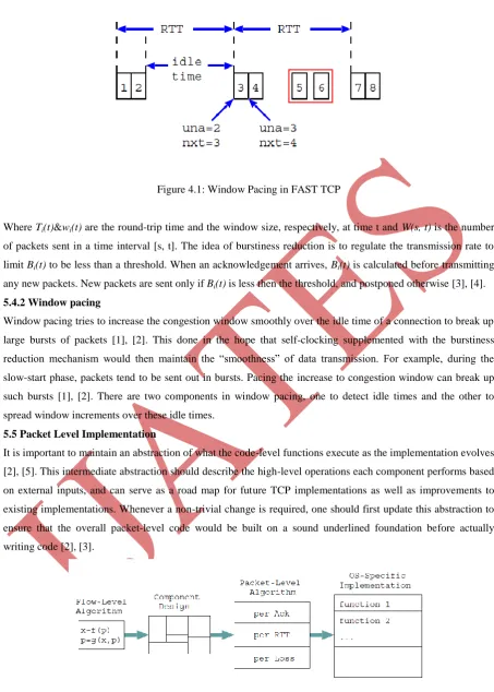
Figure 4.1: Window Pacing in FAST TCP

Where Ti(t)&wi(t) are the round-trip time and the window size, respectively, at time t and W(s, t) is the number

of packets sent in a time interval [s, t]. The idea of burstiness reduction is to regulate the transmission rate to

limit Bi(t) to be less than a threshold. When an acknowledgement arrives, Bi(t) is calculated before transmitting

any new packets. New packets are sent only if Bi(t) is less then the threshold, and postponed otherwise [3], [4].

5.4.2 Window pacing

Window pacing tries to increase the congestion window smoothly over the idle time of a connection to break up

large bursts of packets [1], [2]. This done in the hope that self-clocking supplemented with the burstiness

reduction mechanism would then maintain the “smoothness” of data transmission. For example, during the

slow-start phase, packets tend to be sent out in bursts. Pacing the increase to congestion window can break up

such bursts [1], [2]. There are two components in window pacing, one to detect idle times and the other to

spread window increments over these idle times.

5.5 Packet Level Implementation

It is important to maintain an abstraction of what the code-level functions execute as the implementation evolves

[2], [5]. This intermediate abstraction should describe the high-level operations each component performs based

on external inputs, and can serve as a road map for future TCP implementations as well as improvements to

existing implementations. Whenever a non-trivial change is required, one should first update this abstraction to

ensure that the overall packet-level code would be built on a sound underlined foundation before actually

writing code [2], [3].

Figure 5: From flow-level design to implementation.

Since TCP is an event-based protocol, our control actions should be triggered by the occurrence of various

327 | P a g e

There are four types of events that FAST TCP reacts to: on the reception of an acknowledgement, after the

transmission of packet at the end of an RTT, and for each packet loss.

Figure 5 presents an approach to turn the high-level design of a congestion control algorithm into

implementation. First, an algorithm is designed at the flow-level and analyzed to ensure that it meets the

high-level objectives such as fairness and stability [3], [4].

VI. EQUILIBRIUM AND STABILITY OF WINDOW CONTROL ALGORITHM

In this section we provide a partial analytical evaluation of FAST TCP. We present a model of the window

algorithm. We show that in equilibrium, the vectors of source windows and link queueing delays are the unique

solutions of a pair optimization problems. This completely characterizes the network equilibrium properties

such as throughput, fairness and delay. We also analyze the stability of the control algorithm is locally stable.

Extensive experiments in this section shows its stability in the presence of feedback delay [3], [4], [5], and [6].

VII. PERFORMANCE STUDY OF FAST TCP

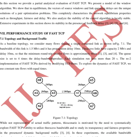
7.1 Topology and Background Traffic

As a baseline topology, we consider many flows sharing a single congested link as shown inFig. 7.1. The

bandwidth of this link is 1.5 Mb/s and it has propagation delay 10ms. Theaccess links have capacity 2 Mb/s and

delay 10ms, so that the minimum round-trip timefor flows is approximately 60ms [1], [3], and [4]. The queue

size is set to 4 times the delay-bandwidthproduct. Each simulation run lasts more than 20 s. The ns-2

implementation of FAST TCPis derived by modifying TCP/Reno. To explore the dynamics of FAST TCP, we

use constant rate flows with equal times.

Figure 7.1: Topology

While not representative of actual traffic patterns, thisscenario is motivated by the need to systematically

explore FAST TCP's ability to utilize theexcess bandwidth and to study its transparency and fairness properties

in the presenceof dynamic background traffic [3], [4]. In these experiments, the available bandwidth

alternatesbetween the full linkscapacities of 1.5 Mb/s when the periodic source is idle.

7.2 Simulation Experiments

We now use simulation based approach to evaluate the performance of FAST TCP in a variety of scenarios,

including FTP, 'square-wave', and other background traffic patterns,with long and short-lived TCP flows on

328 | P a g e

network environments. Weevaluate FAST TCP’s impact on the throughput, fairness, and stability and

responsiveness characteristics of competing cross-traffic [1].

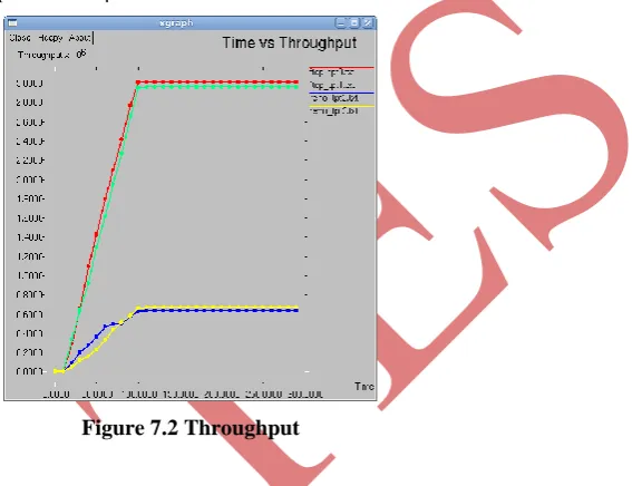
7.2.1Throughput

The average aggregate throughput for the intervalis defined [1], [2]. The system throughput or aggregate

throughput is the sum of the data rates that are delivered to all terminals in a network [6]. Throughput is

essentially synonymous to digital bandwidth consumption; it can be analyzed mathematically by means

of queueing theory, where the load in packets per time unit is denoted arrival rate λ, andthe throughput in

packets per time unit is denoted departure rate μ.

Figure 7.2 Throughput

7.2.2Responsiveness

329 | P a g e

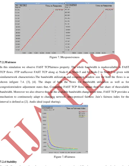
Figure 7.3Responsiveness

7.2.3Fairness

In this simulation we observe FAST TCPfairness property. The whole bandwidth is madeavailable to FAST

TCP flows. FTP trafficover FAST TCP along a) Node-0 to Node-5 and b) Node-2 to Node-7 is given with

similarnetwork characteristics.The bandwidth utilization and congestion window size for both the flows is as

shown infigure 7.4. [3], [4]. The shape of both the flows for bandwidth utilization as well as for

congestionwindow adjustment states that, Competing FAST TCP flows obtain their fair share of theavailable

bandwidth. Moreover we also observe that, as the available bandwidth changesover time, FAST TCP provides a

mechanism to continuously adapt to changing network. Intra-protocol fairness: Jain’s fairness index for the

interval is defined as [2]. Andis ideal (equal sharing).

Figure 7.4Fairness

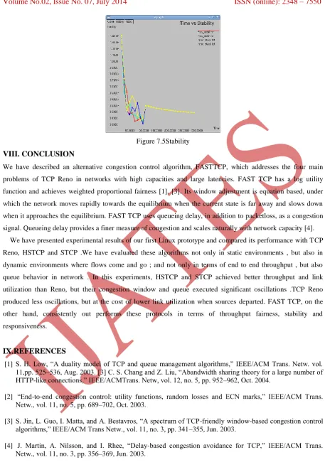
7.2.4 Stability

Specifically, as the number of competing sources in a network, stability become worse for the loss – based

protocols, oscillation in both congestion windows and queue size are more severe all loss base protocols.

Packets loss was more severe. The performance of the FAST TCP did not d grade in any significant way [2],

[3]. Connection sharing the link achieved very similar rates. There was reasonably stable queue at all times, with

little packets loss and high link utilization. Intra protocols fairness is shown in table 4, with no significant

330 | P a g e

Figure 7.5Stability

VIII. CONCLUSION

We have described an alternative congestion control algorithm, FASTTCP, which addresses the four main

problems of TCP Reno in networks with high capacities and large latencies. FAST TCP has a log utility

function and achieves weighted proportional fairness [1], [3]. Its window adjustment is equation based, under

which the network moves rapidly towards the equilibrium when the current state is far away and slows down

when it approaches the equilibrium. FAST TCP uses queueing delay, in addition to packetloss, as a congestion

signal. Queueing delay provides a finer measure of congestion and scales naturally with network capacity [4].

We have presented experimental results of our first Linux prototype and compared its performance with TCP

Reno, HSTCP and STCP .We have evaluated these algorithms not only in static environments , but also in

dynamic environments where flows come and go ; and not only in terms of end to end throughput , but also

queue behavior in network . In this experiments, HSTCP and STCP achieved better throughput and link

utilization than Reno, but their congestion window and queue executed significant oscillations .TCP Reno

produced less oscillations, but at the cost of lower link utilization when sources departed. FAST TCP, on the

other hand, consistently out performs these protocols in terms of throughput fairness, stability and

responsiveness.

IX.REFERENCES

[1] S. H. Low, “A duality model of TCP and queue management algorithms,” IEEE/ACM Trans. Netw. vol. 11,pp. 525–536, Aug. 2003. [3] C. S. Chang and Z. Liu, “Abandwidth sharing theory for a large number of HTTP-like connections,” IEEE/ACMTrans. Netw, vol. 12, no. 5, pp. 952–962, Oct. 2004.

[2] “End-to-end congestion control: utility functions, random losses and ECN marks,” IEEE/ACM Trans. Netw., vol. 11, no. 5, pp. 689–702, Oct. 2003.

[3] S. Jin, L. Guo, I. Matta, and A. Bestavros, “A spectrum of TCP-friendly window-based congestion control algorithms,” IEEE/ACM Trans Netw., vol. 11, no. 3, pp. 341–355, Jun. 2003.

[4] J. Martin, A. Nilsson, and I. Rhee, “Delay-based congestion avoidance for TCP,” IEEE/ACM Trans. Netw., vol. 11, no. 3, pp. 356–369, Jun. 2003.

[5] L. Massoulie and J. Roberts, “Bandwidth sharing: objectives and algorithms,” IEEE/ACM Trans. Netw., vol. 10, no. 3, pp. 320–328, Jun. 2002.