Detection of progression of mastitis by automatic milking systems using neuro-fuzzy networks

(1)

Lincoln University Digital Thesis

Copyright

Statement

The

digital

copy

of

this

thesis

is

protected

by

the

Copyright

Act

1994

(New

Zealand).

This

thesis

may

be

consulted

by

you,

provided

you

comply

with

the

provisions

of

the

Act

and

the

following

conditions

of

use:



you

will

use

the

copy

only

for

the

purposes

of

research

or

private

study



_you

_will

_recognise

_the

_author's

_right

_to

_be

_identified

_as

_the

_author

_of

_the

_thesis

_and

due

acknowledgement

will

be

made

to

the

author

where

appropriate



_you

_will

_obtain

_the

_author's

_permission

_before

_publishing

_any

_material

_from

_the

thesis.

(2)

Detection of Progression of Mastitis by Automatic Milking

Systems using Neuro-Fuzzy Networks

A Thesis Submitted in Partial Fulfilment of the

Requirements for the Degree of

Masters of Software and Information Technology

by

Manishi Kohli

Lincoln University

New Zealand

(3)

~ I ~

Abstract

Mastitis in dairy cattle is the most expensive disease in the dairy industry. It poses a

significant concern to the dairy farmers as it negatively impacts both the milk yield and the

cow health. Various measures have been taken to reduce the occurrence of mastitis including

pre and post milking teat disinfection, good hygiene at milking time, antibiotic therapy etc.

However, these measures have been found effective to a limited extent. Therefore, a need has

been identified for developing a more effective, technology-based mastitis control strategy in

order to have a safe, infection-free and nutritious milk supply. One potential mean of

addressing the mastitis problem is through the use of intelligent computational systems such

as neural and neuro-fuzzy approaches.

A number of studies using neural networks have been conducted in the past. The area of focus

of these studies is the exploitation of neural network concepts such as Self Organizing Maps

(SOM) that determine the health state of a cow in crisp form, i.e., whether the cow is sick or

healthy. However, in many cases, a cow can be neither perfectly healthy nor clinically ill but

falls in an overlapping area (e.g., marginally healthy, very ill, etc.). Also, as of now, the

dynamicity of the problem hasn’t been focused on in these studies. Therefore, this study

hypothesizes that a diagnosis of the health state of cattle in a more realistic fuzzy form than

the current crisp form will be closer to the actual health state. This will further help in the

development of effective treatment strategies leading to improved cow health, increased milk

yield and substantial reduction of income loss.

This study attempts to effectively classify the health state and determine the likelihood of that

health state in cows. Exploiting the data collected by robotic milking stations, the aim is to

specify where the health of a cow lies in the spectrum of Mastitis. To achieve this, the existing

research studies have been extended to another level by incorporating fuzziness into neural

network models.

Self-organizing map is the artificial neural network being used in the study, and three different

fuzzy algorithms have been applied on the results extracted from SOM. Subsequently a

comparative analysis has been done to determine the fuzzy algorithm that is best suited for

(4)

~ II ~

algorithms has been obtained from Ward clustering of SOM. The results obtained have been

justified using statistical methods. The study finally converges to a point, where a “critical

area” or the “transition phase” is identified. This phase indicates the border or a “progressive”

region where the healthy cattle advance towards a sickness stage. Thus, the model shows

success in early identification of mastitis, which could lead to the recovery of cattle and

estimation of the accurate time when the preventive measures need to be taken within the

identified critical area.

The practical implementation of the research might help in saving infected dairy cattle by

timely recognition of the disease and administering the treatment to infected cattle at an early

stage. The quality of cattle would improve and so would the amount of milk they produce.

This would further have an impact on dairy products manufactured from milk. This is not only

valuable from biological perspective with enhanced longevity of cattle and maintaining

diverse gene-pool but also from monetary perspective. The financial losses incurred every

year, due to Mastitis disease, are of mammoth proportions. The research has the potential to

contribute to a reduction of this amount significantly.

Keywords: Artificial Neural Networks, Self-organizing map, Fuzzy clustering, Ward

clustering.

(5)

~ III ~

Acknowledgements

I wish to express my deep gratitude to my supervisor Associate Professor Sandhya

Samarasinghe for her immaculate supervision and guidance throughout the course of the

research. Her valuable support has helped in smooth and conclusive progression of my

project.

I am also grateful to my associate supervisor Prof. Don Kulasiri for extending his support and

encouraging me in completing this program successfully.

I would like to extend my appreciation to the Postgraduate Administrators Douglas Broughton

and Tracey Shields. They have helped me in understanding and navigating all the university

processes at each and every step.

My sincere thanks to my friend Raj Pillai for listening patiently about the progress or failure

encountered throughout the course of the research.

My special thanks to the Lincoln University for giving me the opportunity to make this project

a reality.

Last but not least I would like to thank my family for their continuous support and

well-wishes. This thesis would not have been possible without their encouragement. Their

unwavering faith in my abilities has kept me motivated to achieve the rightful culmination of

(6)

~ IV ~

~ V ~

5.1 Results from SOM………...25

5.2 Results from fuzzy clustering..………28

5.3 Results from ward clustering………...31

5.4 Results from fuzzy SOM………...33

5.5 Validity of the proposes model and its worthiness for practical implementation...38

Chapter 6 Conclusions………..44

(8)

~ VI ~

List of Tables

Table 5.1 Mean and Standard Deviation of the data in the three FCM clusters for the three

input variables………...29

Table 5.2 Mean and Standard Deviation of the data in the three GK clusters for the three input

variables………...………...30

Table 5.3 Mean and Standard Deviation of the data in the three GG clusters for the three input

variables………...………...31

Table 5.4 Ward likelihood index for up to 20 clusters...……….……..32

(9)

~ VII ~

List of Figures

Figure 3.1 Self Organizing Feature Map…………....……….6

Figure 4.1 3D plot of the data…………..………..22

Figure 5.1 SOM results depicting the three-dimensional data projected onto the

two-dimensional map. The U-matrix panel shows the variation in health states, being affected by

necRM, necFD and nyfRM shown in the other three panels………25

Figure 5.2 3D plot of SOM output………..………..27

Figure 5.3 3D plot of clusters obtained from FCM clustering on original data………....……28

Figure 5.4 3D plot of clusters obtained from GK clustering on original data...…………....…29

Figure 5.5 3D plot of clusters obtained from GG clustering on original data...…....…………30

Figure 5.6 Plot of ward likelihood index against number of clusters………....…………33

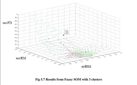
Figure 5.7 Results from fuzzy SOM with 3 clusters………34

(10)

~ VIII ~

Figure 5.9 Results from fuzzy SOM with 13 clusters……….37

Figure 5.10: Track of the health state of a sick cow (Cow ID 212) in the developed mastitis

spectrum………39

Figure 5.11 Track of the health state of a sick cow (Cow ID 316) in the developed mastitis

spectrum………40

spectrum………41

spectrum………42

spectrum………43

(11)

~ 1 ~

Chapter 1 Introduction

Mastitis (Mast: breast, itis: inflammation) is defined as an inflammatory reaction of udder

tissue to bacterial, chemical, thermal or mechanical injury. Mastitis may be infectious caused

by microbial organisms or non-infectious resulting from physical injury to the gland (McGill

University). It is the most expensive disease in dairy industry which costs about 180 million

dollars to New Zealand dairy industry (NMAC Report, 2006). It causes enormous amount of

concern to farmers by negatively impacting milk yield and cow’s health. Mastitis is a very

painful condition which should have declined greatly by now, with improved methods of

prevention. Unfortunately, the incidences of Mastitis have been unacceptably high.

Therefore, the early detection of Mastitis is very important in order to reduce the pain that it

causes to cows and to allow instant treatment which will in turn reduce the economic losses.

Also, it will minimise the chances of other cows getting infected.

Early detection of mastitis can be made possible by capturing the quantitative data of the

traits (as a result of the disease) from automatic milking systems and then by using them to

generate an advanced computational model. Various studies have been undertaken over the

years to create classified health clusters (states) for effective diagnosis of mastitis. Up until

now, three distinct clusters have been identified viz. healthy, moderately ill and severely ill to

classify the dairy cattle for mastitis disease (Sun et al., 2008).

However, not only the diagnosis, but an early diagnosis is very significant in this scenario.

Therefore, a diagnostic tool needs to be generated having the potential of detecting mastitis in

a very initial, sub-clinical mastitis stage. Moreover, this tool should be able to derive the

degree or likelihood of a particular health state of a cow. In an endeavour to make this

possible, in this study, artificial neural network (ANN) has been combined with fuzzy logic

approach.

Artificial neural networks attempt to mimic some of the basic procedures for processing data

as being used by the human brain. These are capable of capturing some of the linear and

non-linear patterns in complex data. Cows suffering from mastitis have higher electrical

(12)

~ 2 ~

Aoki, 1992; Lake, 1992). An ANN could be trained using these traits, and can be expected to

generate useful patterns. Then fuzzy logic can be applied on a well-trained ANN to capture

the fuzzy nature of the health states of a cow. Fuzzy logic deals with the uncertainty of data,

it handles the data which is variable or approximate rather than fixed and exact. Fuzzy logic

will provide an additional flexibility for the cows to be associated with different clusters

(health states). The outcomes of this research can be very confidently used in early diagnosis,

which can initiate an early treatment of mastitis in the dairy industry.

1.1 Objective of Research

The objective of this study is to classify the health state and to determine the likelihood of

that health state in cows affected with mastitis based on neuro-fuzzy approaches. This study

hypothesizes that:

A diagnosis of the health state in a more realistic fuzzy form than in a crisp form will be

closer to the actual health state and in conjunction with its early detection and location in the

mastitis spectrum will help in the development of effective treatment strategies leading to

improved cow health, increased milk yield and reduction of income loss.

Exploiting the data collected by robotic milking stations, the aim is to specify where the

health of a cow lies in the spectrum of Mastitis.

This study aims to test this hypothesis by extending the existing research studies to another

level by incorporating fuzziness into neural network models with a further addition of a

proposed dynamic model. These two aspects are specified as follows.

• As SOM is a deterministic approach, the final output remains crisp. (SOM is a neural

network that implements unsupervised clustering and, in the case of mastitis, can

reveal potential crisp clusters of health states where one cow belongs to a fixed health

state)

• Fuzzy SOMs can be generated by combining fuzzy concepts with SOM. (Fuzzy

concepts can fuzzify the crisp clustering of SOM by making it possible for a cow to

represent several health states to various degrees of likelihood)

(13)

~ 3 ~

model. However, in order to decide which methodology could be the most appropriate and

which could produce the most meaningful outputs, the fuzzy algorithms of interest could be

implemented with the data individually, and an analysis could be made to ascertain which

approach is better. The most fitted approach can then be used with SOM.

1.2 Structure of Thesis

The thesis is organized into six chapters and provides a list of references at the end. A brief

outline of each chapter is presented below:

Chapter 1: Introduction  This chapter provides a brief description about the research area

and identifies the problem. It details the objective and scope of the thesis.

Chapter 2: Background  This chapter provides a detailed description of the mastitis disease

and its economic impact.

Chapter 3: Methods  The ANN, clustering and fuzzy clustering concepts used in the

research has been explained in this chapter. It also provides a survey of literature on the areas

relevant to the research.

Chapter 4: Methodology  This chapter describes the process of implementing the methods

in order to achieve the research objective. In other words, it provides a detailed report of how

the research was carried out.

Chapter 5: Results and Discussion  This chapter illustrates the results in terms of the goals

achieved throughout the research. Also, a discussion of findings has been included in the

same.

Chapter 6: Conclusion This chapter provides a brief description of the problem and how it

has been resolved. Also, it states specific conclusions and sums up all the process and

(14)

~ 4 ~

Chapter 2 Background

Mastitis is a disease resulting from the inflammation of udder (Blowey and Edmondson,

2010). It is defined as an inflammatory reaction of udder tissue to bacterial, chemical, thermal

or mechanical injury (Report from Dept. of Animal Science, McGill University). Mastitis

can be categorised as Sub Clinical Mastitis and Clinical Mastitis. Clinical Mastitis is when

the signs of mastitis are visible such as swollen teat, clotted milk etc. Sub Clinical Mastitis

shows no visible signs, i.e., in this case the udder and milk appear normal.

Mastitis is a very painful condition which should have declined greatly with improved

methods of prevention and treatment (Broom, 2001). However, the incidence of mastitis has

remained unacceptably high. A number of studies since the 1990s report a mean annual

incidence of mastitis ranging from above 30 to over 70 cases per 100 cows (Esslemont and

Kossaibati, 1996; Kossaibati et al., 1998; Esslemont and Kossaibati, 2002, Bradley et al.,

2007).

Inflammation causes changes in the composition of milk from a sick quarter. This includes

increased somatic cell counts (SCC), higher electrical conductivity (EC) and changes in other

components including fat and protein content (Auldist & Hubble, 1998). Somatic cells are

mainly white blood cells sent to fight the infection in the udder. When infection occurs and

starts to damage the udder tissue, the immune system is called into action and, very rapidly,

large quantities of somatic cells are directed to the infection site (Leslie et al., 1983). A report

from Dairy NZ (2006) states that a cow with SCC levels above 150,000 cells /ml is likely to

be infected with mastitis.

As the disease becomes severe, blood-milk barrier is broken and blood (in invisible amounts)

enters milk increasing the EC level in the milk. EC has been widely recognized as an

important indicator of mastitis and employed in mastitis detecting systems in the dairy

industry (Barth et al., 2000). However, in every case, it is not necessary that a cow with high

electrical conductivity would be suffering from Mastitis. Thus, electrical conductivity alone

(15)

~ 5 ~

The economic losses of a clinical case in a default situation were calculated as €210, and vary

from €164 to €235 depending on the month of lactation. The total economic losses of mastitis

(sub clinical and clinical) per cow in a default situation varied between €65 and €182/cow per

year depending on the bulk tank somatic cell count (Huijps et al. 2008). In New Zealand, for

the whole industry, the figure amounts to more than $180 million per year (Bentley et al,

(16)

~ 6 ~

Chapter 3 Methods

3.1 Artificial Neural Networks

Samarasinghe (2006) states that “a neural network is a collection of interconnected neurons

that incrementally learn from their environment to capture essential linear and non-linear

trends in complex data, so that it provides reliable predictions for new situations containing

even noisy and partial information.” There are various ANNs that can be constructed and

used for various purposes. This research study uses Self Organizing Feature Map (SOM)

which is described in next section.

3.2 Self-Organizing Feature Map (SOM)

The competition among the neurons is the mechanism responsible for self-organization in the

brain. This fact is utilized in developing SOM networks shown in Figure 3.1. The process

involves iterative evolution of the network and has two aspects- winner selection and weight

evolution as follows:

Figure 3.1: Self Organizing Feature Map

3.2.1 Selection of winner

The input layer represents the input variables𝑥₁, 𝑥₂…. 𝑥𝑛 for the case of n inputs and each

neuron (circles in Figure 1) is associated with an n-dimensional reference vector 𝑤_𝑖 = [𝑤₁,

𝑤2….𝑤𝑛]. Now the winner selection can be done on the basis of neuron activation or distance

measures.

Each neuron is activated upon receiving an input signal, i.e., an input vector. The activation Neuron Activation

(17)

~ 7 ~

of neuron j is the weighted sum of inputs entering that neuron:

𝑢𝑗 = ∑ 𝑤ni=1 𝑖𝑗𝑥𝑖, [3.1]

where𝑥_𝑖 is ith input variable, wijis the weight connecting input xi and neuron j and 𝑢𝑗 is the

net input which is the weighted sum of inputs 𝑥_𝑖to neuron j.

The neuron havingthe highest activation can be declared the winner. In the natural biological

setting in the brain the winner is found by competition: the output of each neuron𝑢_𝑗is sent as

an inhibitory input signal to other neurons and the process is repeated until one neuron

emerges as the winner with a non-zero 𝑢_𝑗. Computationally, the winner is the neuron with

the highest activation 𝑢_𝑗.

Distance Measure

Euclidean Distance = 𝑑_𝑗 = x - 𝑤𝑗 [3.2]

= �∑ �𝑥𝑛_𝑖=1 _𝑖 − 𝑤_𝑖𝑗�2

The competition would be finally won by the neuron associated with the weight that is closest

to an input (i.e., the smallest Euclidean distance). After the winner selection, unlike in

competitive networks, not only the winner but also neurons in the neighbourhood of the

winner adjust their weights during training. This is an important aspect in the preservation of

spatial organization.

3.2.2 Weight evolution (Learning)

The objective of learning in SOM networks is to accurately project the input data onto the

map neurons. Over repeated exposure to inputs during learning, neurons learn to respond to

inputs in such a way that neurons that are closer on the SOM respond to inputs that are closer

in the actual data space. This feature called topology preservation is achieved by moving not

only the winner neuron but also its neighbour neurons towards the input in order to minimise

the distance between these neurons and the input. In this process, the winner moves by a

larger amount than its neighbours according to a Neighbour Strength (NS) function.

Learning can be illustrated by the following equation:

𝑤𝑗 (t) = 𝑤𝑗 (t - 1) + β (t) NS (d,t) [𝑥(t) - 𝑤𝑗(t - 1)] [3.3]

(18)

~ 8 ~

𝑤𝑗 ( t - 1) is the weight after the previous iteration,

β(t) is the learning rate variation with iterations t,

NS is the neighbour strength function of distance d from the winner to a neighbour neuron at

iteration t, and

𝑥(t) is the input vector presented at the tth iteration.

The learning rate β(t) is user defined and can take the form of linear exponential etc. Starting

with a larger value, β(t) decreases with iterations. NS(d,t) also can be linear, exponential and

Gaussian etc. and shrinks with iterations so that an initially large neighbourhood size gets

reduced to just the winner or winner and its immediate neighbours at the end of the training.

Training stops when there is no acceptable difference in weight adjustment in successive

iterations. The result is a trained map where inputs that are closer in the data space are

projected onto neurons that are closer on the SOM. Therefore, any large gaps between data

in the data space are shown as large distances between corresponding neurons on the map

thereby revealing on the map potential clusters and cluster boundaries in the actual data.

With an appropriate clustering tool, such as Ward Clustering (Section 3.3), neurons that form

clusters on the map can be grouped to form classes for classification purposes. An unknown

input vector then will belong to the class that it is closest to, i.e., the class with the shortest

distance between its mean vector and the input vector. This provides a crisp classification for

the input vector- one input vector belongs to one class.

3.3 Ward Clustering

Ward clustering is an agglomerative clustering method, which was invented in 1963. The

method calculates the distance between the data in clusters and cluster centres by analysing

the variance amongst them. It aims at minimizing the sum of the squares of the distance

between all the data points in a cluster and the centroid of the cluster which was formed as a

result of joining of two clusters. The two clusters that produce the least square distance are

ultimately joined in each step of the process. The distance is calculated as:

d

ward

=

(𝑛𝑟× 𝑛𝑠)

(𝑛𝑟+𝑛𝑠)

||x

r

–x

s

||

2

(19)

~ 9 ~

where r and s, symbolize two clusters and nr & ns are the number of data points in those

clusters. ||xr –xs|| gives the magnitude of the distance between two cluster centres calculated

using Euclidean norm. The ward distance increases with the increase in the number of data

points. The two clusters with minimum dward are joined at each step of this process. The ward

index gives the likelihood of each cluster. The separation of clusters depends upon the value

of the index. The higher the index, more distinctive is the clusters.

Ward Index =

_𝑁𝐶1 × _𝑑𝑑𝑡−𝑑𝑡−1 𝑡−1−𝑑𝑡−2 =

1 𝑁𝐶×

∆𝑑𝑡

∆𝑑𝑡−1 [3.13]

where, ∆dt is the distance between the centres of two clusters to be merged and ∆dt-1 is the

distance between the centres of the clusters merged previously and prior to that step. NC is

the number of clusters remaining. The method is very effective when the dataset is not too

large. Therefore, it is quiet suitable to be used on a trained SOM to cluster map neurons. In

this case, it uses the neuron weights generated by the trained SOM as input vectors.

3.4 Fuzzy SOM

Our aim is to produce a more comprehensive SOM structure by merging it with Fuzzy

concepts. The hypothesis is that it could produce more realistically classified clusters where

each udder reading belongs more to a specific cluster with a degree of membership, thereby,

fuzzifying the crisp boundaries produced by SOM.

There are two ways to approach the above fuzzy classification:

• The first is to create an SOM with the available data. The result of the SOM can then

be fed into an appropriate fuzzy algorithm. This could be done by using the same

number of clusters as produced by the SOM in the fuzzy algorithm.

• The other way is to start with the fuzzy algorithm first. We can try different number

of clusters in it. Comparing all the results we can identify the number of clusters that

give us a fuzzy map which is nearer to our goal of this study. The same number of

(20)

~ 10 ~

Here arises the issue of selecting the most efficient fuzzy algorithm which could be used in

conjunction with SOM. For this, we can work our data with some different and successful

fuzzy algorithms. In the next section we will see how these fuzzy algorithms work.

3.4.1 Fuzzy C- Means (FCM)

The FCM is the most widely used fuzzy clustering algorithm. This technique was developed

by Dunn in 1973 and improved by Bezdek in 1981. It is based on the minimization of the

following objective function:

𝑗𝑚 = ∑ ∑ 𝑢i=1n cj=1 𝑖𝑗m||𝑥𝑖 − 𝑐𝑗||2, 1 ≤ m<∞ [3.4]

where m is any real number greater than 1, 𝑢_𝑖𝑗 is the degree of membership of 𝑥_𝑖 in

the cluster𝑗, 𝑥_𝑖 is the ith d-dimensional measured data vector, 𝑐_𝑗 is the d-dimensional centre

of the cluster j and ||*|| is any norm expressing the similarity between any measured data and

the centre.

Fuzzy partitioning is carried out through an iterative optimization of the objective function

shown above, with update of membership 𝑢_𝑖𝑗 and cluster centres 𝑐_𝑗 . The iteration will stop

when a termination criterion is met.

3.4.2 Gustafson-Kessel Algorithm

The Gustafson-Kessel (GK) algorithm (Gustafson and Kessel 1979) is a powerful clustering

technique. Its main feature is the local adaptation of the distance metric to the shape of the

cluster by estimating the cluster covariance matrix and adapting the distance-inducing matrix

correspondingly.

The GK algorithm is based on iterative optimization of an objective functional of c-means type:

(21)

~ 11 ~

Here, U = [µik] ϵ [0,1]KxNis a fuzzy partition matrix of the data Z ϵ R n x N, V = [v1, v2, … vk],

vi ϵ Rn is a K-tuple of cluster prototypes and m ϵ [1,∞) is a scalar parameter which determines

the fuzziness of resulting clusters. The distance norm DikA, can account for different

geometrical shapes in one data set:

D2ikAi = (zk – vi)T Ai (zk – vi) [3.6]

The metric of each cluster is defined by a local norm-inducing matrix Ai, which is used as one

of the optimization variables in the functional in Eq. 3.5. This allows the distance norm to

adapt to the local topological structure of the data.

3.4.3 Gath-Geva Algorithm

Gath-Geva (GG) clustering algorithm (Gath and Geva, 1989) is based on the minimization of

the sum of weighted squared distances between the data points zk and the cluster centers, vi, i

= 1,….c.

J = (Z; U, V) = ∑𝑐_𝑖=1∑𝑁_𝑗=1(µi,k)mD2ik [3.7]

where V = [v1, v2, … vc] contains the cluster centres and m ϵ [1,∞) is a weighting exponent

that determines the fuzziness of the resulting clusters and m is often chosen to be equal to 2.

The fuzzy partition matrix has to satisfy the following conditions:

U∈ RcxN with µi,k ∈ [0,1], i,k; ∑_𝑖=1𝑐 (µi,k)=1, k; 0< ∑𝑐𝑁_𝑘=1(µi,k) < N, i [3.8]

The distance is calculated based on the fuzzy covariance matrices of the cluster:

(22)

~ 12 ~

The distance function is chosen as

[3.10]

with the a prioriprobability αi

[3.11]

3.5 Use of ANN for Mastitis Diagnosis

Literature on the diagnosis of mastitis in terms of classification of the health state of a cow

using artificial neural networks is not very extensive. However, the amount of research being

done on mastitis is very significant. Early research studies have identified the variables that

are affected by a noticeable amount when a cow suffers from Mastitis. Thereafter, early

1990s saw the beginning of research carried out to exploit neural network techniques to

diagnose mastitis using some or other significant variables. The following review summarizes

some significant research work addressing mastitis diagnosis in chronological order.

1994: NIELEN ET AL.

In the research carried out by Nielen et al. (1994), three analysis techniques were compared

over four models for detection of Clinical Mastitis. The three analysis techniques were

Principal Component Analysis (PCA), Logistic Regression Model (LRM) and Neural

Network model (NNM). The four models were generated by producing different

combinations of input variables. The input variables used in this research were milk

production, milk temperature and electrical conductivity (EC). No preprocessing was

performed on EC data; it was used as it accounts for biological effects as explained before.

The definition of clinical and sub clinical quarters were stated by farmers who could observe

it on the basis of various visible factors.

(23)

~ 13 ~

mastitis. For this, PCs were plotted against each other in two dimensional plots. If a

separation between the clinical and healthy quarters occurred, the variation present in the two

components was assumed to be caused by mastitis. LRM & Back propagation neural network

(NN) models were trained to differentiate between healthy and clinical quarters. In LRM 2x2

contingency matrix was used and in NN a three layered feed forward network was used.

PCA explained 90% of the variation for two models and 80% of variation for the other two.

LRM produced 84% sensitivity and 90% specificity where sensitivity is the percentage of

correct classification of mastitis quarter and specificity is the percentage of correct

classification of healthy quarters. Three layered back propagation neural network model

produced 84% sensitivity and 97% specificity. All three models showed almost similar

performance, but NN showed slightly better performance than LRM.

Also, the same three techniques were used to develop models based on data for two prior

milking, i.e., the data extracted just before a cow got signs of mastitis. The LRM and NN

models showed 70% sensitivity and 90% specificity, which mean that not in every instance

clinical mastitis could be observed before clinical signs emerge as deviations are not very

clear always.

1995: NIELEN ET AL.

In this research, artificial neural network techniques were used for diagnosis of sub clinical

mastitis (SCM). The authors used back propagation neural networks to classify healthy and

sub clinical quarters. This research used a three layered feed forward network, with one

output unit which stated 0 for healthy quarters and 1 for sub clinical quarters. The inputs used

for this model were milk production which was calculated using an exponential smoothing

function. Parity (1 and >1) and days in milking were other inputs and the final input used was

electrical conductivity.

They defined a healthy period when a cow’s somatic cell count (SCC) is < 200 x 103 cells/ml.

As soon as the cow’s SCC exceeds this figure, the healthy period was terminated. Period for

severe sub clinical mastitis was defined when cow’s SCC > 1000 x 103 cells/ml and moderate

SCM was between 500 and 1000 x 103 cells/ml. Periods which didn’t fall under the above

(24)

~ 14 ~

In this analysis, a period of 14 milkings was chosen with consideration. They defined

sensitivity as a measure for detecting a sub-clinical cow and specificity as a measure for a

healthy cow. For training, a random number of healthy cow milkings were chosen in such a

way that data contains almost equal numbers of healthy and sub-clinical milkings. The full

model consisted of 15 inputs (which were derived from the four basic inputs as mentioned

above), 7 hidden neurons and 1 output neuron.

Sensitivity obtained was 66% and specificity obtained for 14 healthy milkings was 80%. In

the same research, logistic regression model was also used with the same input parameters

which produced sensitivity of 54% and specificity of 92%. They concluded that neural

network model could be trained to be specific or sensitive but never to be both according to

the outputs obtained during training. Also, they highlighted that a low sensitivity of EC to

detect periods of high SCC could be a result of the fact that EC and SCC are related to udder

health but are less related to each other. But they also remarked that this will have only a

slight effect on neural network model as correlated variables are not significant for this

model.

1999: YANG ET AL.

In the work carried out by Yang et al. (1999), neural networks were exploited to distinguish

between the clinical and healthy quarters. They used a number of variables including SCC,

lactation number, milk yield, days in milking, mean SCC for herd, season of calving, herd

size, milk components etc. and the complete dataset had 0.33% of clinical mastitis cases

compared to the total number of records. Three datasets were then created with ratios of 1:1,

1:10 and 1:300 mastitis records: non mastitis records.

The trained network achieved 83% accuracy in distinguishing between clinical and healthy

cows. Also it was observed that 1:1 ratio dataset performed better than the other datasets.

2003: LOPEZ-BENAVIDES ET AL.

In the research carried out by Lopez-Benavides et al. (2003), the state of progression of

(25)

~ 15 ~

taken at weekly intervals for 14 weeks and they were observed for electrical conductivity,

somatic cell count, fat percentage and protein percentage. But new informative variables were

used to train the network. New variables included inter-quarter ratio (IQR), conductivity

index (CI), linear score (SCS) and composite milk index (CMI). IQR and CI were derived

from EC values. SCS is a linear transformation of SCC and CMI is the sum of the values of

all the raw and derived milk traits. Electrical conductivity and CMI were used as inputs and

SOM clustered the dataset into previously undefined healthy, moderately ill, ill and severely

ill health categories. A deep investigation into the clusters revealed that the SOM categorized

the data into significant health categories. They also stated that the combination of

moderately and severely ill health categories could be investigated further, as it might

produce improved results. CI, EC and CMI were the most important indicators of the

mastitis status.

2005: WANG AND SAMARASINGHE

In the work performed by Wang and Samarasinghe (2005), the data included the milking data

collected by automated milking systems over a four month period from four farms. In this

research, preprocessing of data played a significant role. The variables were normalized and

final variables used were normalized peak electrical conductivity (EcMax), normalized

quarter yield fraction and maximum relative deviation of EcMax values among four quarters

for a cow. Specifically, these respective variables were running mean of normalized electrical

conductivity and running mean of normalized quarter yield and fractional deviation from the

smallest normalized electrical conductivity value.

The dataset produced after normalization was used to construct SOM artificial neural

networks model. Due to the presence of only 3% mastitis cases in the total number of records,

five random datasets were generated to balance the ratio of sick to healthy cows to some

extent. All neural network models displayed 94% sensitivity and 100% specificity on

average. In order to assess the robustness of the results, three fold cross validation was

exploited over 3 self-organizing maps and 95% sensitivity and 97% specificity was realized.

2008: KRIETER ET AL.

(26)

~ 16 ~

generated using electrical conductivity of milk, milk production rate, milk flow rate and days

in milking as input data. They set the block sensitivity (threshold for generating an alert) in

training data to be at-least 80%. The specificity (percentage of mastitis cases recognized) was

recorded as 61.4% and 78.3% for two different definitions of Mastitis and the error rates were

46.5% and 79.1%. They concluded that more detection parameters can help in obtaining more

accurate results.

2009: SUN ET AL.

In the work carried out by Sun et al. in 2009, multi-layer perceptron and self-organizing

feature map were used to detect mastitis in cows from data collected by automated milking

systems. They also used the same variables as those used in Wang et al. (2005), i.e., running

mean of normalized electrical conductivity and running mean of normalized quarter yield and

fractional deviation from the smallest normalized electrical conductivity value. However, the

raw data for the study came from readings from cows diagnosed as clinically ill.

Specifically, readings from these cows from the date of diagnosis back to the point where

they were healthy were assembled into a dataset for all sick cows. This way, the data set

contained information for the whole mastitis spectrum - from healthy through stages of

mastitis up to clinical mastitis. Mastitis was defined as follows: if the quarter milking samples

had 12.8% drop in milk yield and 15% higher than average of the two lowest quarters in

electrical conductivity value, then the quarter has mastitis. According to this definition, they

generated a new data set which had 4.6:1 healthy to sick quarter’s ratio.

Sun et al. (2009) and Sun (2008) report that a thorough investigation of raw electrical

conductivity quarter readings clearly demonstrated that not all infected quarters have the

highest electrical conductivity and lowest milk yield in an udder. Hence four different input

combinations were used amongst which one was formed by using principal components for

addressing multi co-linearity in the data. The PC based MLP model showed better

performance compared to the other models. It had the highest overall correct classification

rate of 90.75%, with sensitivity of 86.90% and specificity 91.35%. The SOM classified the

stage of progression of mastitis into three clusters: healthy, moderately ill and severely ill.

The clusters obtained were validated using K-means clustering, ANOVA and least significant

difference. This research stated that the relatively low sensitivity rate could be the result of

(27)

~ 17 ~

model can be used to detect mastitis of a cow and SOM can be used to visualize the health

status of the cow for early diagnosis and treatment. This SOM can also be used to assess the

overall health status of a herd for better management of the herd.

It is worth noting here that our study is a direct extension of Sun et al. (2009) work using

their data. Sun et al. (2009) classified cow health state into 3 categories and we aim to

represent a more refined mastitis spectrum in a model using the same data and build on it a

decision making system. A more complete description of data and inputs are presented in the

Methods section.

3.6 Use of Fuzzy Logic in Mastitis Diagnosis

There are very limited numbers of research studies which have used fuzzy logic for detection

of mastitis. However, the results produced from these studies have been obtained from

practical implementation on automatic milking systems, hence making the conclusions very

significant. The studies are explained in the following section.

2001: MOL ET AL.

In the work carried out by Mol et al. (2001), the information from the sensors which measure

milk yield, temperature of the milk, electrical conductivity of the milk were used. The aim of

this study was to reduce the false-positive cases. False-positive cases can be defined as those

cases which got a positive mastitis alert from the system but they were not afflicted with the

disease. This study used fuzzy logic to develop a model which could produce alerts in an

automated system. The data traits used were yield, temperature, electrical conductivity of the

milk and activity of each cow. Based on these traits, a fuzzy inference system was developed

which followed three steps to complete the process.

In the first step, the fuzzification of the variables was performed, i.e., the real time variables

were transformed into linguistic variables. In the second step, if…then rules were generated,

using linguistic variables. These rules were grouped into rule boxes. In the third step,

defuzzification was performed. Now, the linguistic variables are translated back to real

(28)

~ 18 ~

Using this approach the false-positive alerts were reduced from 1266 to 64. Mol et al. (2001)

stated that “classification by a fuzzy logic model proved to be very useful in increasing the

applicability of automated cow status monitoring”.

2006: CAVERO ET AL.

The aim of the research carried out by Cavero et al. (2006) was to develop a fuzzy model to

classify and control mastitis in dairy cows. The data used for this research was collected by

University of Keil’s experimental dairy farm “Karkendamm”. 478 cows were used to collect

the data. Mastitis was identified according to three different definitions. These were: (1)

udder treatments, (2) udder treatment or somatic cell counts (SCC) over 100,000/ml and (3)

udder treatment or SCC over 400,000/ml. The data traits used were electrical conductivity,

milk production rate and milk flow rate.

A multivariate model was used in this study to improve the detection of mastitis. The data

obtained from sensors was used as input data for a fuzzy model. A fuzzy inference system

was generated using same process (fuzzification, fuzzy inference, and defuzzification) as

explained in the previous section. They used random test and training data and set the block

sensitivity to at-least 80%. The specificities obtained were between 93.9% and 75.8% and the

error rate varied between 95.5% and 41.9% depending on mastitis definition. The average

number of true-positive cases obtained per day was 0.1 to 7.2 and the average number of false

positive cases per day varied from 2.4 to 5.2 where the average size of herd data was 39.7

cows per day.

They concluded that fuzzy logic is a very efficient approach for this application. The results

obtained showed that the model could be generalized. The error rate could be decreased

(29)

~ 19 ~

Chapter 4 Methodology

This chapter describes the methods used to meet the research objectives of the study. It is a

two stage approach, which puts special emphasis on the data analysis and model

development. In the first stage the data has been observed carefully, so that it could be

efficiently exploited in the model development stage. In the modeling stage,

• SOM, which is an ANN, is trained, and the results obtained are compared with those

from Sun et al. (2009) study.

• Three fuzzy algorithms, namely Fuzzy C Means, Gustafson-Kessel and Gath Geva,

are applied on the original data.

• Ward clustering is performed in order to obtain the optimum number of clusters on

SOM.

• SOM obtained above (step 1) is being used to create the fuzzy SOM using the best

selected fuzzy algorithm (step 2), and the number of clusters to be generated has been

selected using Ward clustering (step 3). Thus a fuzzy SOM is developed at this stage

of the research.

4.1 Data Analysis

Already pre-processed data from Sun et al. (2009) study is used for this research. A brief

description of the data is as follows.

The data were supplied by Dairy NZ, which has been collected from 194 cows by an

automated milking system, constituting 48,546 records from late July 2006 to early April

2007. Although there were a large number of records, as explained previously, the raw data

for the study came from readings from cows diagnosed as clinically ill. Specifically, readings

from these cows from the date of diagnosis back to the point where they were healthy were

assembled into a dataset for all sick cows. These data were augmented with data from

healthy cows to complete the dataset. This way, the data set contained information for the

(30)

~ 20 ~

For this study, as in Sun et al. (2009), mastitis was defined as follows: if the quarter milking

samples had 12.8% drop in milk yield and 15% higher than average of the two lowest

quarters in electrical conductivity value, then the quarter has mastitis. As the data originally

contained a very small number of mastitis cases compared to healthy cases, it was assumed

that the results will be highly dominated by healthy cases, thus neglecting the features of

mastitis cases. Hence, a new dataset was created in which there were a total of 4128 quarters

and the ratio of healthy to sick samples approximated 4.6:1.

The variables used for our study are the same as those in Sun et al. (2009) study and these

are: running means of normalized quarter yield fraction (nyfRM) for each quarter, running

means of normalized electrical conductivity (necRM) for each quarter, and fractional

deviation from the smallest necRM value (necFD) for each quarter. The detail derivation of

these variables is as follows:

Running means of normalized quarter-yield fractions (nyfRM)

This variable is calculated in two steps. First step involved the calculation of quarter yield

fraction (QYF) which is the ratio of milk yield of a quarter in a milking to the total milk yield

from all four quarters from that milking. Biologically, this variable accounts for all the

variations in the milk yield between each quarter of each cow. In the case of mastitis, the

sick quarter can be expected to have a lower QYF than the healthy quarters.

Second step involved calculating running means of QYF. It was based on correction of QYF

as per the following equation:

𝑥′𝑡 = 𝑥𝑡 �_𝑎1�+ (1−1_𝑎)𝑥𝑡−1 [4.0]

where𝑥′_𝑡is the running mean of QYF at time t, 𝑥_𝑡 is the measured QYF at time t, 𝑥_𝑡−1 is the

measured QYF at time t −1 and a is a coefficient that represents ‘running mean length’.

The running mean of QYF was calculated at two levels:

(31)

~ 21 ~

ii) Quarter level: This was calculated for individual quarters over their own history

of milking. The value of a was set as 5 at this level.

Now, the quarter running mean of QYF was divided by its corresponding herd running mean

of QYF to obtain the Running Means of Normalized Quarter-yield Fraction for each quarter

of each cow at each milking. This normalization was adopted in order to correct some

machine problems which occur time and again.

Running Means of Normalized Electrical Conductivity (necRM)

This variable was calculated using electrical conductivity of milk, in the same way, as

nyfRM.

Fractional deviations from the smallest necRM value (necFD)

This variable was created to consider the ratio of the three highest necRM values to the

lowest one. It was calculated as

necFDi = necRM_necRMi−necRMmin

min [4.1]

where necFDi is necFD of any of the four quarters of a cow, necRMi is normalized EC

running mean (necRM) of the same quarter, and necRMmin is the smallest value of necRM

between four quarters. This variable is used because the health condition of a cow is not the

same in all four quarters in mastitis, and larger fractional deviation can be expected when a

cow is sick. Therefore, necRMmin is the value of the electrical conductivity when the cow is

in its healthiest stage. Hence, necFDi generates a very high value for an infected case

(32)

~ 22 ~

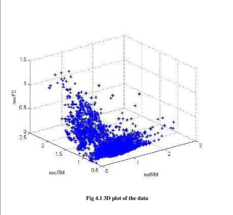
Fig 4.1 3D plot of the data

Figure 4.1 shows a plot of the data used in this study which shows that sick quarters in

general have high electrical conductivity (i.e., high necFD and necRM) and low milk yield

(i.e., nyfRM) and vice versa. As can be seen, the data covers the whole mastitis spectrum

form healthy to clinical mastitis; thus the data satisfy the requirement of a model that is going

to use them to make a representation the whole spectrum.

4.2 Model Development

This section highlights all the techniques which have been used in this study to develop the

(33)

~ 23 ~

4.2.1 Development of SOM

Thus each input vector for SOM is of 3 dimensions, necFD, necRM and nyfRM. As SOM is

an unsupervised (clustering) network, there is no output variable. The SOM toolbox2

(Alhoniemi et al., 1999) is used to develop the SOM model and the number of neurons is

calculated as

Units = ceil [5 × dlen0.5] [4.2]

where dlen is the number of records in data and ceil is the ceiling function. The number of

records in the data used is 4128; hence, using equation [4.2], the number of neurons obtained

is 322. To use a more convenient number of neurons, 325 have been used to develop this

model. As the original dataset contains 4128 records, 325 neurons is assumed to be a

sufficient size to represent our data.

Sun et al. (2009) in fact developed an SOM for this data using commercial neural networks

software and their SOM was supposed to be the starting point for our study as our work is an

extension of Sun et al. (2009) study to take it to a higher level of capability. However, as our

study aims to go deeper into the mastitis spectrum, we need to delve deep into the best

possible cluster granularity to build our extended model. Sun et al. (2009) used three clusters

but we need to check all possible clusters. Nonetheless, Sun et al. (2009) could be used as a

benchmark for this data as we proceed with the same data into deeper horizons.

4.2.2 Fuzzy Clustering

Clustering divides the data points in such a way, that data-points in one cluster are as similar

as possible and those in different clusters are as dissimilar as possible. In crisp or hard

clustering, a data-point is fixed with one cluster but in fuzzy clustering one data-point can

belong to more than one cluster with a different membership level associated with each

cluster which describes the degree of belonging of a data-point to a cluster.

In this study, three fuzzy algorithms have been applied to our data. These three algorithms are

Fuzzy C Means, Gustafson Kessel and Gath geva. A comparison has been made between the

outputs from these algorithms to select the best suited algorithm for this application. Further,

in a quest to verify the topological preservation made by SOM, all the algorithms have also

(34)

~ 24 ~

4.2.3 Ward Clustering

A novel aspect of our study is the attempt to dig into the intricacies of mastitis progression.

With the aim to obtain a more refined mastitis spectrum, an important issue that arises here is

“what number of distinct health regions or clusters can give us the greatest insight”. In order

to resolve this problem, ward clustering has been adopted. It uses the SOM output (i.e.,

neuron weights) as input data and gives an index value to the number of all possible clusters.

The higher the index value, the more likely is the distinctiveness of that particular number of

clusters. The optimum number of clusters thus formed on the SOM can be thought of as

covering the mastitis spectrum in terms of likely distinct transitions of health states as cow

health moves from healthy to clinical mastitis.

4.2.4 Fuzzy SOM

Using the best selected fuzzy algorithm, and the number of clusters as being proposed by

ward clustering, a fuzzy SOM is generated over the data produced by SOM. Initially, a visual

comparison is made about how the different number of clusters affects the application. Then,

some interpretations are made for the fuzzy SOM with ‘n’ number of clusters which has the

highest likelihood in ward clustering. In a fuzzy SOM, a cow belongs to all the clusters but

have different degree of membership values for each cluster. The higher the degree of

membership value, the higher is the association of the cow in that particular cluster.

(35)

~ 25 ~

Chapter 5 Results and Discussion

5.1 Results from SOM

A SOM with 325 neurons was trained to get an initial picture of data distribution and how

individual variables affect the health state. The number of neurons used for training of SOM

was selected as per Eq. 4.2 as explained in Section 4.3.1. Three input variables were used,

i.e., nyfRM, necRM and necFD, in the input layer of this network and these are the

normalised quarter running mean of: yield fraction, electrical conductivity and fractional

deviation of EC, respectively. The Gaussian function was used as the neighbourhood

function and the initial learning rate used was 0.5.

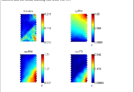
Fig. 5.1: SOM results depicting the three-dimensional data projected onto the two-dimensional

map. The U-matrix panel shows the variation in health states, being affected by necRM, necFD

(36)

~ 26 ~

In Fig. 5.1, the U-matrix shows the variation in health states with respect to the combined

effect of all the three variables. The other three panels depict the variation in individual

variables. The location of neurons in the panels corresponds to each other making it possible

to assess the correspondence of variables to each other and to the health state. As an SOM is

a condensed version of the data, each neuron is the centre of gravity of a cluster of inputs.

The whole map therefore, preserves the probability density distribution of the actual data. In

the three panels showing the individual variables, blue colour depicts lower values and red

colour depicts higher values. The two panels for necRM and necFD show strong

correspondence as can be expected since they both depict versions of EC. Also, very high

yield fraction, red area in the nyfRM panel, relates to quite low values of necRM and necFD

showing that the SOM has captured the generally accepted trends among the three variables.

In the U-matrix, colour depicts the distance between adjacent neurons on the map; blue

colour indicates smaller distances indicating areas of tighter clustering and red colour

indicates areas with larger neuron distances indicating either loosely formed clusters or

cluster boundaries. Accordingly, the large bright blue section in the U-matrix represents a

reasonably tight cluster of healthy cows because it could be easily observed that the top left

sections in necRM and necFD panels have the lowest values and the same section in the

nyfRM panel is covered by relatively high values thus making that area in the U-matrix

dominated by healthy cases. The top right section is populated by cows with very high yield

(nyfRM) and pretty low EC (necRM and necFD). However, the red colour in the U-matrix in

the corresponding top left region indicates large distance between neurons. This means that

cows with extremely high yield associated with very low EC (i.e., extremely healthy state)

may be too few and are relatively far from each other to form a tight cluster. It may mean

that such values are not the norm for a typical healthy state.

The bottom right section of U-matrix also shows a red region where neurons are relatively far

from each other. This area is dominated by the highest EC in the necRM and necFD panels

and moderately high yield in the nyfRM panel. Therefore, this region is where very sick

cows are represented and they are more spread out in the data space as indicated by the red

colour in the U-matrix compared to the tightly knit large blue healthy cluster. The presence

of less mastitis cases in data (1 to 4.6 healthy cases) justifies this. Also, Wang and

Samarasinghe (2005) who analysed sick and healthy cow data based on the same 3 inputs as

in our study showed that the healthy data form a much tighter cluster compared to the more

(37)

~ 27 ~

case is higher than for a healthy case. However, it could be seen that not always a sick cow

has the highest EC (necRM and necFD) values and the lowest yield (nyfRM) value. This

gives an insight about the fact that there is a peculiar and unique relationship between these

variables, which couldn’t be stated as directly or inversely proportional with respect to the

health state. This gives a very strong reason to explore the spectrum that a cow might be

following while progressing with the disease, and also when changing these variables

abruptly in some or other way. U-matrix shows neuron distances ranging from dark blue and

light blue to red, there appears to be some progressive health stages in the health state

spectrum that could be revealed by formally clustering map neurons, which is the topic of the

next section.

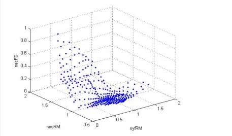
Fig 5.2 3D plot of SOM output (i.e., neuron weights corresponding to the three input variables)

Figure 5.2 shows the 3D plot of SOM weight vectors (SOM output). On comparing this plot

with the plot of the original data in figure 4.1, it can be observed that SOM has preserved the

topological nature of the data, removing the noise. The justification of removal of noise from

the data by SOM will be discussed later in this chapter. Thus, this ‘preservation’, supports the

argument that SOM has treated the data fairly taking into account spatial relations and

probability distribution of the data and improves our confidence to take the SOM to the next

(38)

~ 28 ~

5.2 Results from Fuzzy Clustering

In this section, results from the three selected fuzzy algorithms are presented in terms of how

they cluster the original data. Also a comparative study has been performed, in order to

select the best suited fuzzy algorithm for the “mastitis application” which could be used

further in the research. For fuzzy clustering, the number of clusters needs to be

predetermined. Based on the results from the previous research of Sun et al. (2009), three is

the number of clusters used in fuzzy clustering. The input variables used are the same as

those used in Section 5.1 for the development of SOM. First of all, fuzzy c means is used for

performing fuzzy clustering over the data. The value of the weighting component which

determines the fuzziness of the clusters is set to 2 and termination tolerance is 1e-6. Fig. 5.3

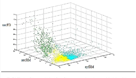
shows the 3D plot of fuzzy c means clustering of the data. Three clusters were obtained as

denoted by three different colours in the picture. The black circles in every cluster represent

the cluster centre. The sky blue cluster is the healthy cluster, yellow cluster represents the

moderately ill health stage and green cluster represents the ill health stage. This assessment of

health stages was done by making an analysis of the data traits being used. For example, a

high yield- low electrical conductivity-low fractional deviation of electrical conductivity is

healthy stage whereas the reverse shows an ill health stage.

Fig 5.3 3D plot of clusters obtained from fuzzy c means clustering on original data (blue-

(39)

~ 29 ~

Table 5.1 shows the mean and standard deviation values of the data for all the three FCM

clusters for the three variables. The values are significantly different proving the clusters to

be distinctive and important.

Table 5.1 Mean and Standard Deviation of the data in the three FCM clusters for the three

input variables

Variable Health Category

Healthy Moderately Ill Severely Ill

nyfRM 1.2303±0.2392 0.7379±0.1852 0.4122±0.2836

necRM 0.9924±0.1350 0.9951±0.1149 1.4115±0.1935

necFD 0.0622±0.0890 0.0460±0.0478 0.4383±0.2168

Now, keeping the values of the number of clusters, membership function and termination

tolerance same, Gustafson Kessel (GK) clustering was performed. In Gath Geva (GG)

clustering the only modified value was termination tolerance which was set as 1e-4. The

results obtained are presented further in this section. Next explained is GK clustering.

Figure 5.4 show the plot obtained using the same data, data traits and other parameters by

performing GK clustering. The description of the figure is same as that of Fig 5.3; the blue

cluster represents healthy, yellow – moderately ill and green – ill health.

Fig

5.4 3D plot of clusters obtained from GK clustering (blue- healthy; yellow- moderately ill;

(40)

~ 30 ~

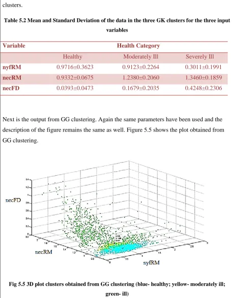
Table 5.2 shows the values of mean and standard deviation of the data in all the three GK

clusters.

Table 5.2 Mean and Standard Deviation of the data in the three GK clusters for the three input

variables

nyfRM 0.9716±0.3623 0.9123±0.2264 0.3011±0.1991

necRM 0.9332±0.0675 1.2380±0.2060 1.3460±0.1859

necFD 0.0393±0.0473 0.1679±0.2035 0.4248±0.2306

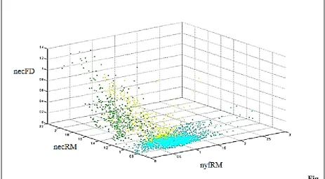
Next is the output from GG clustering. Again the same parameters have been used and the

description of the figure remains the same as well. Figure 5.5 shows the plot obtained from

GG clustering.

Fig5.5 3D plot clusters obtained from GG clustering (blue- healthy; yellow- moderately ill;

green- ill)

(41)

~ 31 ~

Table 5.3 Mean and Standard Deviation of the data in the three GG clusters for the three input

variables

nyfRM 0.9509±0.3150 0.9240±0.2185 0.6669±0.4697

necRM 0.9195±0.0554 1.0882±0.0370 1.3027±0.2271

necFD 0.0264±0.0265 0.0188±0.0191 0.3391±0.2201

The fuzzy c means clusters as shown in Figure 5.3 are very distinct and less intermingling or

overlapping than GK and GG clusters. In GK clusters as shown in Figure 5.4, the moderately

ill and ill health states are highly overlapping, which gives rises to the increasing probability

of not distinguishing the health states very clearly. GG clustering shows a very little

moderately ill region, which again creates a difficulty in identifying the spectrum of the

health states. Thus, keeping the main objective in mind, which is figuring out the health

spectrum, the fuzzy c means clustering was found to be the most suitable for the application,

as it very clearly distinguishes the three clusters which were asked. But still the health

spectrum is not very clearly visible. This causes an urge to look further into the optimum

number of clusters which are needed to be generated in order to obtain a clear movement of a

cow through various health stages. This could give a very transparent picture of a cow

transitioning from a healthy stage towards the sick health state.

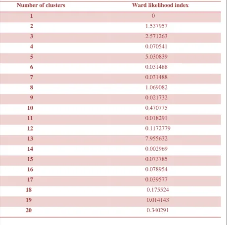
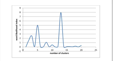
5.3 Results from Ward Clustering

As observed in Section 5.2, there is still a need for exploring the optimum number of clusters

in order to meet our objective of obtaining the health spectrum in a more refined and useful

way. Ward clustering was being opted here, to address this situation. Ward clustering is

capable of providing the number of clusters that could be distinctively extracted from a