Honors Theses and Capstones Student Scholarship
Spring 2019
Determination of Multi-Messenger Signals from
Matter Outflows of Merger Systems
Ronny Nguyen
UNH Department of Physics
Follow this and additional works at:https://scholars.unh.edu/honors
Part of theAtomic, Molecular and Optical Physics Commons,Cosmology, Relativity, and Gravity Commons,Nuclear Commons,Physical Processes Commons, and theStars, Interstellar Medium and the Galaxy Commons
This Senior Honors Thesis is brought to you for free and open access by the Student Scholarship at University of New Hampshire Scholars' Repository. It has been accepted for inclusion in Honors Theses and Capstones by an authorized administrator of University of New Hampshire Scholars' Repository. For more information, please [email protected].
Recommended Citation
Nguyen, Ronny, "Determination of Multi-Messenger Signals from Matter Outflows of Merger Systems" (2019).Honors Theses and Capstones. 472.
Matter Outflows of Merger Systems
Ronny Nguyen
Advisors: Francois Foucart, Harald Kucharek
University of New Hampshire Department of Physics
UNH Institute for the Study of Earth, Oceans, and Space
∗
In 2017, LIGO detected gravitational waves from GW170817. This presented for the first time, gravitational waves originating from a neutron star - neutron star merger. Studies of neutron star mergers are significant because the multi-messenger signals in the form of gravitational waves and electromagnetic waves can inform us on the nuclear physics of neutron stars and the creation of heavy elements in the universe. Matter is ejected in the merging process and forms the outflow which provides a neutron-rich environment for rapid neutron capture (r-process) to occur leading to the nucleosynthesis of heavy elements. What we detect on Earth are kilo-nova emissions powered by the radioactive decays of these heavy, unstable elements. Therefore, simulations that accurately model the time evolution of matter outflows are needed to study neutron star mergers. In this study I have performed a sim-ulation of a binary neutron star merger using the SpEC-Hydro code. The merger system consists of a 1.2Mand 1.4M neutron star which are counter-rotating with respect to one another. With data from the simulation I used classical mechanics (accounting for relativistic corrections) to recreate the time evolution of particle tra-jectories in order to model the matter density distribution at any arbitrary time. This method is not limited to binary neutron star mergers and can be applied to any generic merger system. I will also be covering the work I have done in [1] regarding neutrino transport schemes. We used a Monte-Carlo (MC) algorithm to analytically solve Boltzmann’s equations of radiation transport. I analyzed the neutrinos emitted by a binary neutron star merger remnant and compared the neutrino distribution function of the MC scheme to a two-moment scheme.
CONTENTS
I. Background 4
A. Recent Developments in Multi-Messenger Astronomy 4
1. Gravitational Waves - A Brief Introduction 4
2. 2015 LIGO/Virgo Detection of GW150914 5
3. 2017 Joint Detection of GW170817 and GRB170817A 5
B. Neutron Star Merger Physics 6
1. Evolution and Outflow Processes 6
2. Neutrino Transport 8
II. Methods 9
A. Neutron Star Merger Simulation 9
B. Neutrino Transport using a Monte-Carlo Algorithm 10
C. Matter Density Distribution 10
D. Particle Trajectories 11
III. Results 12
A. Evolving the Neutron Star Merger Simulation 12
B. Recreating the Matter Density Distribution 14
C. Angular Distributions 14
1. Matter Distribution 14
2. M1 and MC Neutrino Distributions 15
IV. Conclusions and Discussion 16
V. Acknowledgments 18
I. BACKGROUND
A. Recent Developments in Multi-Messenger Astronomy
1. Gravitational Waves - A Brief Introduction
One of the core tenants of general relativity is that all objects in the universe possessing
energy creates a curvature in spacetime. Gravitational waves are the ripples in curved
spacetime caused by massive objects in motion. These ripples transport energy in the form
of gravitational radiation and propagate at the speed of light. While any object with energy
can produce gravitational waves, these signals are extremely weak and negligible for most
systems. The strongest sources of gravitational waves that we are able to detect are from
astronomical stellar events such as binary neutron star mergers, black hole mergers, and
supernovae. Other events such as the big bang and early universe formation may also
possibly be able to be studied with this new medium. Even with these stellar events as
references in the search for ripples in spacetime, gravitational waves still prove difficult to
detect with only a handful being published in the past 4 years. The difficulty of detecting
gravitational waves comes from the weak interaction of the gravitational force, being a factor
of 10−36 weaker than the electromagnetic force. However, by the same virtue of this weak interaction are we able to detect these signals because gravity is also a long range interaction
that propagates across spacetime. When gravitational waves are produced by a stellar
event, absorbing the radiant energy in the form of gravitational radiation is difficult. This
is an advantageous property that gravitational waves have over other forms observational
mediums such as electromagnetic waves. Therefore, gravitational waves allows us to observe
objects in locations where electromagnetic signals would otherwise be absorbed or dispersed.
In summation, the nature of gravitational waves provides a window into the universe
by allowing us a medium in which to study the formation of the early universe shortly
after the big bang, the formation of heavy elements, and stellar evolution. Perhaps more
importantly, gravitational waves provides a confirmation on the theory of general relativity
2. 2015 LIGO/Virgo Detection of GW150914
On September 14, 2015, the LIGO and Virgo collaborations detected gravitational waves
from a binary black hole merger designated GW150914. This constituted the first ever
observation of gravitational waves and demonstrated the existence of binary black hole
systems [2]. LIGO and Virgo confirmed this detection by matching the observed data from
the black hole merger to gravitational wave templates created by simulations. Moving
forward from the match made by simulations against the black hole merger data, LIGO and
Virgo proceeded to plot the strain amplitude vs. time as well as the frequency vs. time
(refer to Fig. 1 in [2] for visualization of graph). As the black hole binaries began spiraling
inwards towards each other, the frequency of the signal begins to increase until the two
objects merge together. This increase in frequency leads to what is commonly referred to
as the “chirping” of the gravitational wave signal because the pitch increases along with
frequency.
With real world data now available to the scientific community, numerical simulations of
merger systems such as that performed by SpEC-Hydro, a relativistic hydrodynamics code,
have taken on and have been an integral part in verifying gravitational wave detections. At
the time of this writing, a total of 11 gravitational wave detections have been published from
black hole mergers. Neutron star mergers have since also been adding on to these numbers.
A variety of other theoretical sources such as neutron star - black hole mergers are currently
undergoing studies but have so far not been detected yet.
3. 2017 Joint Detection of GW170817 and GRB170817A
On August 2017, the LIGO and Virgo collaboration detected a gravitational wave signal
from GW170817 [3]. This detection was an important event for two reasons. First, it marked
the first time gravitational waves were detected originating from a binary neutron star merger
and second, the Fermi Gamma-ray Space Telescope reported a gamma-ray burst from the
same source 1 second prior to the gravitational wave detection. The gamma-ray burst was
later designated as GRB170817A. The joint detection from LIGO/Virgo and Fermi was the
first time an electromagnetic counterpart to a gravitational wave source was observed [4].
being real. Follow up studies to the LIGO/Virgo and Fermi detection confirmed that the
electromagnetic counterpart detection was a kilonova which are optical and infrared signals
from radioactive decay of unstable elements [5] [6]. The electromagnetic counterpart to
GW170817 in particular was significant because it was an indication for the presence of
matter and a confirmation of a neutron star source. The presence of matter is significant
in determining the composition of the matter outflows and how the system evolves. The
composition of matter will in turn change the composition of kilonova emissions that we
detect on Earth. Kilonova emissions are created by the nuclear reactions that occur in
the matter outflow. Rapid neutron capture by atomic nuclei results in the nucleosynthesis
of heavy elements which then undergo radioactive decay into stable elements. It is the
radioactive decay of these heavy elements in the outflow that powers kilonova emissions [7].
LIGO and Virgo inferred the masses of the neutron stars in the binary system to be
between 1.17 – 1.60M with a total mass of 2.74+0−0..0401M. The masses of the neutron stars I
used to for the SpEC simulation were 1.2M and 1.4M with the total mass of the system
being 2.6M which is typical of neutron star mergers in the Milky Way. The model in this
thesis differs from the GW170817 observation in that we have set both neutron stars to
be counter-rotating whereas the neutron stars of GW170817 were not. This sets the stage
for the analysis of possible future detections that have rotation in the system. Developing
accurate models of neutron star merger system is essential because we use the modeled data
and compare it to data from actual detections. The primary results of this thesis recreates
the matter density distribution at any arbitrary time after merging which allows us to see
how the system evolves over long period of time thus giving us an insight into the nuclear
processes responsible for kilonova signals originating from neutron star mergers.
B. Neutron Star Merger Physics
1. Evolution and Outflow Processes
Binary neutron star mergers are phenomena where a neutron star is engaged in an inward
spiral with another neutron star. As the orbits of the bodies get smaller, the orbital period
decreases while tidal forces increases. The tidal forces that the neutron stars exert on each
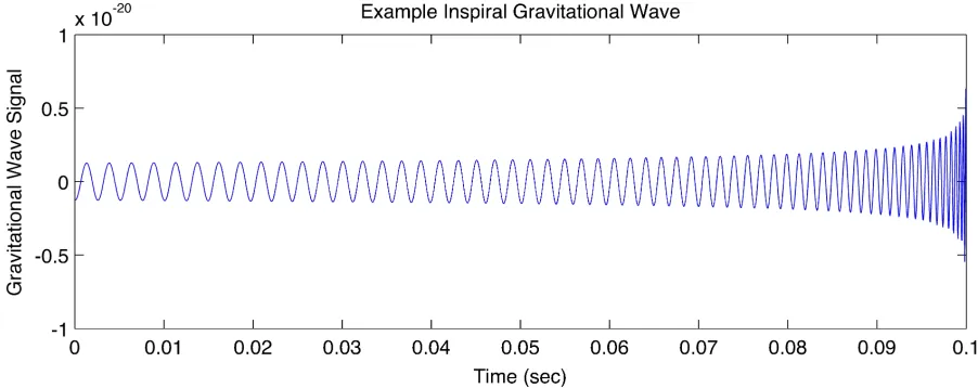
plotted from the data of our SpEC simulation. The frequency of the gravitational wave also
increases rapidly as the orbits decrease. This is known as the “chirp” of a gravitational wave
which is visualized in Fig. 1.
FIG. 1: The “chirping” of a generic gravitational wave. The frequency increases as the
orbits of the binary merger objects gets smaller until they eventually merge together. All
credit goes to A. Stuver of the LIGO collaboration for the publication this plot [2].
Using gravitational wave signals we can extrapolate the masses, spins and radii of the
merger objects (albeit with large uncertainties for the spins and radii). With this information
we can calculate the mass ratio of a merger system,
q= m2
m1
(1)
where m1 and m2 are the masses of the neutron stars and m1 ≥ m2. The mass ratio
of GW170817 was 0.7–1.0 with a total mass of the system being 2.74+0−0..0401M [3] which is
consistent with the population of neutron star binaries observed in the galaxy. We now
have two ways in which we can identify the source objects of a gravitational wave – first
by observing an electromagnetic counterpart (an indication of the presence of matter in
the ejecta) and second by observing the mass ratio. Determining the size of the bodies
in a merger system (particularly in neutron star mergers) is of interested to us because it
gives us information on the composition and the size of the cores of the merger objects thus
When the neutron stars collide two tidal tails form which eject matter. The matter can
either be bounded and accrete which forms the disk around the post-merger object [8] [9] or
become unbounded which forms the outflow of matter leaving the system. Inside the matter
outflow, rapid neutron capture (r-process) occurs between neutrons, protons, and electrons
resulting in the nucleosynthesis and creation of heavy elements. The heavy elements then
undergo radioactive decay into stable elements which we observe on Earth. Entropy increases
in the outflow while the temperature decreases due to the expansion of heated matter.
The ejected matter in the outflow significantly influences the optical emissions that are
able to be detected. The mass of the ejecta determines the longevity of a kilonova emission
– more mass being present results in brighter and longer emissions. The speed of the ejected
matter will change the timescale of the emission as well. In terms of composition, more
neutrons present results in emissions that are visible in the infrared spectrum while less
neutrons results optical emissions.
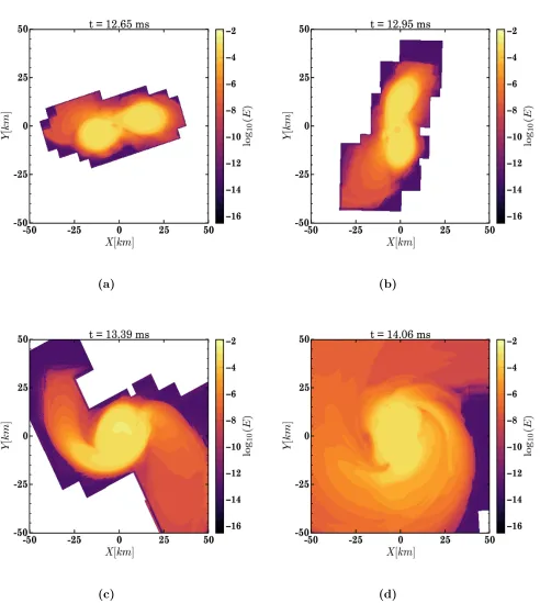
After collision, the two neutron stars begin to merge into one singular object which is
visualized in Fig. 3c and 3d. At this point in the evolution the cores of the neutron stars
have completely merged while matter continues to be ejected and accreted around the
post-merger object.
2. Neutrino Transport
Neutrinos play an important role in the composition of the matter outflows of neutron
star mergers. First, nucleosynthesis is dependent on the number of neutrons and protons
in the outflow – neutrinos are directly coupled to the number of these nucleons through
absorption and emission. Protons and neutrons can capture neutrinos which changes the
amount of each nucleon in the outflow. This becomes significant in the r-process that
occurs; without a neutron-rich environment, neutron capture becomes less prevalent. As
previously discussed, neutron capture results in the formation of heavy elements. Less
neutrons leads to lower mass elements that are still unstable and undergo radioactive decay.
Lower mass elements have a lower optical depth which allows photons to escape earlier in the
merger evolution when matter in the outflow is hotter. Neutron-poor environments caused
by neutrino absorption leads to kilonova emissions at higher temperatures and frequencies
thermal emissions due to lower rates of radioactive decay, neutrinos take part in cooling of
the post-remnant object by the following reactions,
n + e+ →p + ¯ν
p + e− →n +ν.
(2)
Neutrino treatments such as that used by [1] and [10] utilizes a full general relativistic
model of neutron star mergers with an approximate neutrino transport scheme. These
treatments use a two-moment scheme which includes the energy density J,
momentum-density H, and stress-energy tensor S. These are known as the 0th, 1st, and 2nd moments
respectively. They are explicitly written as momentum-space integrals as follows,
J(νi) =
Z
dνν3
Z
dΩf(νi)
H(µν
i) =
Z
dνν3
Z
dΩf(νi)l
µ
S(µνν
i) =
Z
dνν3
Z
dΩf(νi)l
µ
lν.
(3)
Where f(νi) is the neutrino distribution function in momentum space, l
µ and lν are the
direction of propagation of the neutrinos with respect to the 4-velocity of the fluid, and ν
is the neutrino energy in the fluid frame. The two-moment scheme is used to couple the
evolution of neutrinos to the fluid. It should be noted that we are not given all the variables
needed to close the system of equations and because of this we choose our own analytical
closure called M1 in [1]. Further discussion of the closure along with my previous work is
discussed in further detail in Sec. II B.
II. METHODS
A. Neutron Star Merger Simulation
In this study I simulated a counter-rotating binary neutron star merger consisting of
1.2M and 1.4M neutron stars. This simulation was created using SpEC-Hydro, a
rela-tivistic hydrodynamics code [11], [12]. SpEC creates a set numerical grid where the
simula-tion takes place. We ran the simulasimula-tion first on the Trillian computer cluster at the UNH
Blue Waters computer cluster at the University of Illinois for further computational needs
as the neutron star merger simulation evolved. The neutron stars begin at a distance of 50
km a part with initial orbital velocities of 0.12c. Each neutron star is also counter-rotating
with respect to the direction of their orbits. The SpEC simulation allowed me to observe
directly (with returned data) the evolution of the neutron star merger at different phases. I
show the results of the simulation in Fig. 3at different timestamps.
B. Neutrino Transport using a Monte-Carlo Algorithm
As part of this thesis I will discuss the work of a previous paper I have worked on [1].
This work pertained to neutrino transport using two different methods, the two-moment
scheme with M1 closure and a newly developed MC algorithm (at the time of writing). The
system we applied these methods to was another binary neutron star merger. I developed
models for the analysis for neutrinos in the matter outflow for both methods. Specifically, I
analyzed the energy distribution of neutrinos as well as their angular distributions. In this
study I used the same method for analyzing the angular distribution of matter particles in
my neutron star merger simulation.
In [1],J andHin Eq. 3were evolved and we chose an analytical closure forS to close the
system of equations which we call M1. We used an MC algorithm to solve for Boltzmann’s
equations of radiation transport and compare it to the two-moment scheme with the M1
closure. As previously mentioned in Sec. I B 2, the two-moment scheme is what couples
neutrino evolution to the fluid so what closure we use to close the system of equations will
impact the evolution of the neutron star merger.
C. Matter Density Distribution
SpEC outputs relevant data that I used to recreate the matter density distribution. It
creates a numerical grid which is set where the simulation takes place. I want to analyze the
evolution of the system beyond the grid boundary and so to do this I modeled the trajectory
of particles using Newton’s law of gravitation and Kepler orbits conditions. It should be
noted that by modeling the particles using classical mechanics that our velocities are in
would have implications with the initial conditions of the trajectories, (x0, y0, z0, vx0, vy0, vz0).
Therefore, I perform a linear transformation to ensure that energy is conserved between the
classical and relativistic results. This returns the approximated relativistic velocities. With
the relativistic velocities set, we use Newton’s law of gravitation which is integrated resulting
in a 6D coupled differential equation. I solved this coupled system of six differential equations
numerically using the approximated six initial conditions (x0, y0, z0, vx0,gr, vy0,gr, vz0,gr). This
returned the trajectory of each particle as a function of time which I used to recreate the
matter distribution for any arbitrary time in the future.
D. Particle Trajectories
To recreate the trajectory of particles we use data sampled at the boundary of the SpEc
numerical grid. This provided us with six initial conditions (x0, y0, z0, vx0, vy0, vz0) that
allowed us to evolve the system. We modeled the particles leaving the grid using Newton’s
law of gravitation,
~
Fgrav =m~r¨=
−GM m
r3 ~r. (4)
Where M is the summed mass of the neutron stars, m is the mass of the particle in the
outflow, G is the Newtonian gravitational constant, and ~r(x, y, z) is the variable we solved
for. Integrating this equation results in a 6D coupled differential equation. We wanted to
see the evolution of x, y, z, vx, vy, and vz so we solved the system of differential equations
for these variables numerically with Python. However, it must be noted that SpEC is
a relativistic code but we modeled the particles trajectories using Newtonian mechanics.
Therefore, if we want to accurately model the evolution of the neutron star merger system
then we have to make a linear transformation to reconcile the discrepancies between our
classical and relativistic results. To accomplish this, we looked at conservation of energy,
(Av)2
2 −
GM
r =−Ut−1. (5)
On the left-hand side is the classical model with kinetic and potential energy terms.
On the right-hand side is the SpEC relativistic model where −Ut is the conserved specific
rest mass energy (mc2). A is the linear transformation term that is applied to the particle
velocities. Solving for A gives
A= r
2 −Ut+GM/r−1
v2
. (6)
We then applied the transformation term A to the velocitiesv of each modeled particle,
(Av)2 = (Avx)2+ (Avy)2+ (Avz)2
=v2x,gr+v2y,r+v2z,gr.
(7)
The second line in Eq. 7 are the obtained relativistic velocities. With these relativistic
velocities we now have the approximated initial conditions needed to numerically evolve the
system; (x0, y0, z0, vx0, vy0, vz0) → (x0, y0, z0, vx0,gr, vy0,gr, vz0,gr).
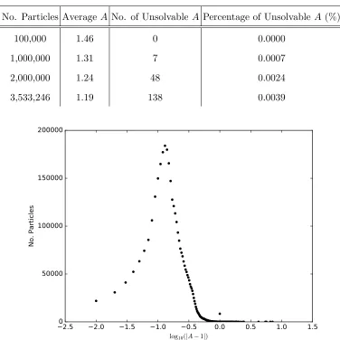
We visualized the correction factor A in Fig. 2 and found that the majority of particles
only needed a ∼10% correction. This can also be seen in Table I – as more particles were
sampled, the correction factor decreased. This was because the first hundred thousand or
so particles are close to the merger system which introduced large errors on the orders of
2–3. Later particles are farther away from the system and have a lower error. Some particle
velocities could not be transformed into relativistic velocities due the fundamentally different
metric in classical and relativistic mechanics. What this meant was that the classical energies
in Eq. 5 could not be reconciled with the relativistic energies from SpEC. This resulted in
the radicand in Eq. 6 to become negative and the value to be imaginary. We found that
only ∼0.0039% out of the 3.5 million simulated particles could not be reconciled.
III. RESULTS
A. Evolving the Neutron Star Merger Simulation
Using SpEC, we recorded the matter density of the system as it was evolved. This allows
us to graph the matter density and directly observe the evolution of the matter outflow at
different stages in the simulation. Fig. 3 shows the evolution of the binary neutron star
system at 12.65, 12.95, 13.39, and 14.06 ms. In Fig. 3a the tidal forces start to deform
the shapes of both objects. We see that the neutron stars begin to merge into one singular
TABLE I: Properties of the relativistic correction factorA used to ensure that energy is
conserved in our classical and relativistic simulations. We see that as more particles are
sampled that the correction factor decreases. This is because earlier particles are much
more closer to the merger itself which results in errors. Unsolvable A values are due to the
radicand of the square root in Eq. 6becoming negative at certain values. This is due the
different metrics in classical and relativistic mechanics.
No. Particles AverageA No. of Unsolvable A Percentage of Unsolvable A (%)
100,000 1.46 0 0.0000
1,000,000 1.31 7 0.0007
2,000,000 1.24 48 0.0024
3,533,246 1.19 138 0.0039
−2.5 −2.0 −1.5 −1.0 −0.5 0.0 0.5 1.0 1.5
log10(|A − 1|)
0 50000 100000 150000 200000
N
o.
Pa
rt
ic
le
s
FIG. 2: Correction factor A to transform our classical velocities to relativistic velocities.
The peak near -1.0 indicates that the majority of particles roughly needed ∼10%
correction.
of the neutron stars begin to merge together as seen in Fig. 3c and the overall shape of the
system starts to resemble one object instead of two. It is important to notice the two tidal
eject more and more matter over time and form the accretion disk around the post-merger
object which Fig. 3d shows. The ejected matter from the tidal tails also forms the matter
outflow which we used to sample particles for our classical model in Sec. II D.
B. Recreating the Matter Density Distribution
In Sec. II D we recreated the trajectories of particles from classical mechanics while also
making a correction to ensure that energy is conserved between the classical and relativistic
results. We are now in a position to model the matter density distribution of particles at
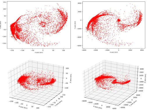
an arbitrary time in the future. Fig. 4 shows the evolution of particles at 1 ms and 37
ms after merging. Fig. 5 serves as a better visualization of the evolution of the system at
various timestamps. Here the axes are set to give the reader a better sense of the distance
the outflowing particles travel. We considered the bound conditions of particles using Eq. 5
as follows:
= (Av) 2
2 −
GM
r . (8)
If < 0 the particle is bounded and if > 0 the particles is unbounded. We are
interested in the evolution of particles for a short time in the evolution. This is because
unbound particle trajectories form a hyperbola and over long distances they will simply be
a straight line. Bound particles will remain orbiting the post-merger object. We found that
82% of the 3.5 million particles were bound while 17% were unbound. Only 6 particles had
= 0 which are parabolic orbits. Unbound particles are more interesting to us because they
are what power kilonovae.
C. Angular Distributions
1. Matter Distribution
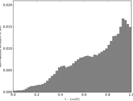
The angular distribution of particles impacts the observable properties of kilonovae. Fig.
6 shows the angular distribution of particles using a spherical coordinate system. We use
the following equation to calculate the angle at which particles leave the system with respect
θ= arctan s
x2+y2
|z2|
(9)
We observe that the majority of particles leave at angles further away from the polar
regions (θ >30◦). Around the polar region (θ < 30◦), matter was not abundantly present. We found most of the matter leaving the merger system around the equatorial plane. This
matter dominated region will be optically dense which will not allow for photons to pass
through the matter outflow and leave the merger system in the these directions. This is
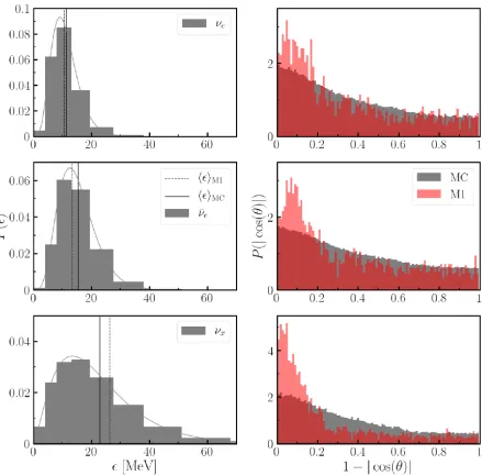
in agreement with the angular distribution of neutrinos in Fig. 7 (Fig. 8 in [1]) where it
was observed that the neutrinos (not the matter particles) were mostly focused in the polar
region. Although the M1 closure overestimates the abundance of neutrinos in the polar
region, we observed that even in the MC plot that there is a greater amount of neutrinos in
the this region than around the equatorial plane. The presence of neutrinos will result in the
polar region being optically thin due to radioactive decay of less massive unstable elements
which we discussed in Sec. I B 2. In summation, photons from kilonova emissions will be less
likely to pass through optically dense regions near the equatorial plane due to absorption
and dispersion from the matter particles. However, we note that the equatorial ejecta will
only be optically thick on a timescale of days after merging but eventually becomes optically
thin within a timescale of weeks [13]. When this happens, most of the energy of the kilonova
will come from the equatorial ejecta.
2. M1 and MC Neutrino Distributions
We found with the M1 analytical closure that there was a large inaccuracy to actual
neutron star merger models in the regions close to the polar axis (θ < 30◦). This resulted to a ∼50% overestimation of neutrinos in those regions. We surmise these regions to be more
optically thin than leading to more photons passing through the matter outflow resulting in
the kilonova to have a higher frequency emission which is the same process that we previously
discussed when optically thick regions turn optically thin over time. Despite this, we found
that the M1 closure performed well elsewhere. When we obtained the neutrino distribution
with the MC algorithm we did not encounter the same overabundance of neutrinos in the
polar regions as with the M1 closure which can be seen in Fig. 7.
scheme can improve upon current two-moment schemes. First, with a low resolution MC
simulation we can forgo the need to use the M1 closure which resulted in large inaccuracies
in the polar regions. This is done by using time-averaged moments as a closure for the
two-moment scheme. From using time-averaged moments, we found that distribution of
neutrinos was only weakly dependent on the time evolution. This allows our time-averaged
MC simulations to be comparable to that of dynamically evolved systems. Second, the MC
methods presented in [1] hints towards the viability of using an MC closure. Replacing the
M1 closure with the MC closure in two-moment schemes can in principle reduce numerical
errors by an order of magnitude for the current number MC packets that we can currently
afford computationally.
IV. CONCLUSIONS AND DISCUSSION
In this thesis I have presented a methodology to recreate the matter density
distribu-tion of particles at any arbitrary time using classical mechanics and then making a linear
transformation to reconcile with relativistic mechanics. Although the simulation I ran was a
binary neutron star merger the method presented in this thesis can be applied to any generic
binary merger system such as black hole mergers.
In making the linear transformation from classical and relativistic velocities I found that
there were some particles that could not be reconciled to match that of our SpEC
simu-lation. These irreconcilable particles comprised ∼ 1.7% of the 3.5 million particles in the
simulation. The irreconcilable particles were due to the fundamentally different metric used
in classical and relativistic mechanics. In addition, abnormally large transformation
fac-tors, A, on the order or 2 – 3 were because the first few hundred thousand particles were
close to the merger system. As I sampled particles further away I found that the
correc-tion factor decreased with the majority only needing a ∼10% correction. After performing
the transformation from classical to relativistic mechanics, I obtained six initial conditions
(x0, y0, z0, vx0,gr, vy0,gr, vz0,gr) which I used to solve for the particle motion numerically after
integrating Newton’s law of gravitation. This gave the trajectories of the particles which
allowed me to model the matter density distribution at any arbitrary time. The matter
density distribution is plotted in Figs. 4and 5.
methods as in [1]. I found that particles were leaving at angles further away from the polar
region (θ > 30◦) and near the equatorial plane. This was where the accretion disk formed and where most of the matter outflow was present. The matter dominated regions results
in r-process and where the creation of heavy elements takes place (heavier than elements
created in neutron-poor environments). Radioactive decay of heavy elements results in an
optically thick region around the equatorial plane where electromagnetic emissions from
kilonovae is suppressed. However, this changes as the system continues to evolve. The
equatorial ejecta is thick on a timescale of days after merging occurs. After a timescale of a
week or so, the optically thick region becomes optically thin enough for kilonova emissions to
penetrate through the ejecta. This has an affect of changing the composition of the kilonova
– the late time emissions comes at lower temperatures due to cooling in the outflow.
Using returned data from the SpEC neutron star simulation, I created matter density
plots. This allowed me to directly observe the evolution of the system at different timestamps
in the simulation. From Fig. 3a and Fig. 3b I observed the deformation in the shape of the
neutron stars due to tidal forces. The tidal tail that begins to form in Fig. 3c ejects matter
which creates the matter outflow. The merging of the neutron star cores also occurs at this
time and in Fig. 3c and 3d the post-merger object is formed while matter continues to to
be ejected and accreted.
Finally, I have discussed the work I have done with neutrino transport in [1] and
elabo-rated on the significance of the role of neutrinos in the evolution of neutron star mergers.
We compared a newly developed MC simulation to a two-moment scheme that used the M1
closure. We saw that using the M1 closure resulted in an overestimation of neutrinos in
the polar region (θ < 30◦) by ∼ 50% while performing well everywhere else. The overesti-mation of neutrinos in the polar regions changes the properties of the kilonova by reducing
the amount of neutrons and protons through absorption. Consequentially, the polar regions
become a neutron-poor environment. While the nucleosynthesis of heavy elements will still
occur via r-process, these elements will have less mass compared to heavy elements in a
neutron-rich environment. The radioactive decay of these less massive heavy elements
re-sults in an optically thin region that photons can pass through. This a similar (but not
entirely the same) process that happens when the optically thick regions of the matter
out-flow become optically thin – the kilonova emission will occur from a higher temperature
on the other hand did not have the issue of neutrino overestimation in the polar regions.
The comparison between the MC and two-moment scheme can be seen in Fig. 7.
Despite the errors of the M1 closure, we surmised that MC simulations can improve
upon current two-moment schemes in two ways. First, the MC method provides a way
to forgo the use of M1 closures by using low resolution MC simulations thus reducing the
large inaccuracies in the polar regions. This was done by using time-averaged moments for
the two-moment scheme. Therefore, our MC simulations can potentially be comparable to
simulations that are dynamically evolved. Second, the MC method presents the possibility
of using an MC closure to reduce numerical errors that plague the M1 closure by an order
of magnitude.
V. ACKNOWLEDGMENTS
First and foremost I would like to express my gratitude to Dr. Foucart for his
mentor-ship throughout this project and the opportunity to partake in research in computational
astrophysics for the past 2 years. I would also like to thank the members of Dr. Foucart’s
research group Alexander Chernoglazov, Alexander Knight, and Christian Krueger for being
the most jovial people I have had the pleasure to work with and know. Acknowledgments
also go to the UNH Institute for the Study of Earth Oceans and Space for the use of the
Tril-lian computer cluster as well as the University of Illinois and NSF for the use and funding
[1] Foucart F, Duez M D, Kidder L E, Nguyen R, Pfeiffer H P, and Scheel M A. Evaluating radiation transport errors in merger simulations using a Monte Carlo algorithm. Phys. Rev. D, 98:063007, Sep 2018.
[2] Abbott B P, Abbott R, and Abbott T D. Observation of Gravitational Waves from a Binary Black Hole Merger. Phys. Rev. Lett., 116:061102, Feb 2016.
[3] Abbott B P, Abbott R, and Abbott T D. Gw170817: Observation of gravitational waves from a binary neutron star inspiral. Phys. Rev. Lett., 119:161101, Oct 2017.
[4] Abbott B P, Abbott R, and Abbott T D. Multi-messenger Observations of a Binary Neutron Star Merger. Astrophys. J., 848(2):L12, Oct 2017.
[5] Smartt S J, Chen T W, and Jerkstrand. A kilonova as the electromagnetic counterpart to a gravitational-wave source. Nature (London), 551(7678):75–79, Nov 2017.
[6] Valenti S, Sand D J, Yang S, Cappellaro E, Tartaglia L, Corsi A, Jha S W, Reichart D E, Hais-lip J, and Kouprianov V. The Discovery of the Electromagnetic Counterpart of GW170817: Kilonova AT 2017gfo/DLT17ck. Astrophys. J., 848(2):L24, Oct 2017.
[7] Metzger B D. Kilonovae. Living Reviews in Relativity, 20(1):3, May 2017.
[8] Radice D, Perego A, Hotokezaka K, Fromm S A, Bernuzzi S, and Roberts L F. Binary Neutron Star Mergers: Mass Ejection, Electromagnetic Counterparts, and Nucleosynthesis. Astrophys. J., 869(2):130, Dec 2018.
[9] Fernandez R, Tchekhovskoy A, Quataert E, Foucart F, and Kasen D. Long-term GRMHD simulations of neutron star merger accretion discs: implications for electromagnetic counter-parts. , 482(3):3373–3393, Jan 2019.
[10] Wanajo S, Sekiguchi Y, Nishimura N, Kiuchi K, Kyutoku K, and Shibata M. Production of all the r-process nuclides in the dynamical ejecta of neutron star mergers. The Astrophysical
Journal, 789(2):L39, Jun 2014.
[11] Duez M D, Foucart F, Kidder L E, Pfeiffer H P, Scheel M A, and Teukolsky S A. Evolving black hole-neutron star binaries in general relativity using pseudospectral and finite difference methods. Phys. Rev. D, 78(10):104015, Nov 2008.
Equation of state and spin orientation effects. Phys. Rev. D, 87(8):084006, Apr 2013.
(a) (b)
(c) (d)
FIG. 3: Density map of neutron star model at various stages of evolution after the
beginning of merging together. (a) Shows the neutron stars before merging completely.
(b) The cores of the neutron stars begin to coalesce into a single compact object. (c) At
this point the cores have almost completely merged together. Matter from the tidal tail
begins to whipped away from the system. (d) As the system continues to evolve, matter
FIG. 4: Time evolution of particles 1 ms (LHS) after merging and 37 ms (RHS) after
merging. Top images provides a 2D view of the system while the bottom images provides a
3D view. 82% of the 3.5 million simulated particles were bound with <0 while 17% were
unbound with >0. We found only 6 particles with= 0 . After merging, the ejected
particles continue to move at a fraction of c which can be seen with the difference in order
(a) 1 ms (b) 8.5 ms
(c) 26 ms (d) 37 ms
FIG. 5: Set axes visualization of the time evolution of particles 1, 8.5, 26, and 37 ms after
0.0
0.2
0.4
0.6
0.8
1.0
1 − |cos(θ)|0.000
0.005
0.010
0.015
0.020
No
rm
ali
ze
d A
mo
un
t in
Bi
n
FIG. 6: Angle distribution of particles leaving the merger system. Particles leave the
system as angles further away from the polar angle (z-axis). This allows the emission of
kilonova signals around the optically thin polar region with less matter that can
FIG. 7: The left column shows the energy distribution of neutrinos leaving the SpEC
numerical grid for 3 neutrino species: electron neutrinos νe, electron antineutrinos ¯νe, and
heavy-lepton neutrinos νx. The dashed vertical line shows the neutrino energy estimated
by the M1 scheme, and the solid vertical line is the neutrino energy estimated by the MC
scheme. The right column shows the angular distribution of neutrinos leaving the grid.
The overestimation of neutrinos in the polar regions by the red M1 scheme is visually
evident when compared to the grey MC scheme. For all of these plots the neutrino fluxes