ISSN: 2231-5381
http://www.ijettjournal.org
Page 4459Fuzzy Model Reference Learning Control For
Non-Linear Spherical Tank Process
S.Ramesh#1 and S.Abraham Lincon#2 #1
Department of Electronics and Instrumentation Engineering, Annamalai University, Annamalai nagar-608002, Tamil nadu, India.
Abstract Fuzzy Model Reference Learning Control
(FMRLC) is an efficient technique for the control of non linear process. In this paper, a FMRLC is applied in to a non linear spherical tank system. First, the mathematical model of the spherical tank level system is derived and simulation runs are carried out by considering the FMRLC in a closed loop. A similar test runs are also carried out with Neural Network based IMC PI and conventional ZN based PI-mode for comparison analysis. The results clearly indicate that the incorporation of FMRLC in the control loop in spherical tank system provides a good tracking performance than the NNIMC and conventional PI mode.
Keywords FMRLC, FOPDT, NNIMC, ZN PI
I. INTRODUCTION
Control of non linear process is main criteria in the process control industries. This kind of nonlinear process exhibit many not easy control problems due to their non-linear dynamic behavior, uncertain and time varying parameters. Especially, control of a level in a spherical tank is vital, because the change in shape gives rise to the non-linear characteristics. An evaluation of a controller using variable transformation proposed by Anathanatrajan [1] on hemi-spherical tank which shows a better response than PI controller. A simple PI controller design method has been proposed by Wang and Shao [2] that achieves high performance for a wide range of linear self-regulating processes. Later in this research field, Fuzzy control is a practical alternative for a variety of challenging control applications, since it provides a convenient method for constructing nonlinear controllers via the use of heuristic information. Procyk and Mamdani [3] have discussed the advantage of Fuzzy Logic Controllers (FLC) is that it can be applied to plants that are difficult to get the mathematical model. Recently, Fuzzy logic and conventional control design methods have been combined to design a Proportional Integral Fuzzy Logic Controller (PIFLC). Tang and Mulholland [4] have discussed about the comparison of fuzzy logic with conventional controller.
Recent years, neural network (NN) had been adopted in nonlinear IMC design due to its good ability of approximate arbitrarily nonlinear vector
functions [5][6]. For some complex processes, however, when the work condition of system varies, the process characteristic changes drastically and falls outside training region. Even though the NN model is available, it is difficult to design the NN inverse controller unless the model is open-loop stable [7]. When the process is unstable in local region, the controller based on a fixed model will be unreliable and thus the system performance is affected seriously.
To trounce these problems, in this paper a “learning” control algorithm is presented which helps to resolve some of the issues of fuzzy controller design and NN inverse model. This algorithm employs a reference model (a model of how you would like the plant to behave) to provide closed-loop performance feedback for synthesizing and
tuning a fuzzy controller’s knowledge-base.
Consequently, this algorithm is referred to as a “Fuzzy Model Reference Learning Controller” (FMRLC) [8][9][10].
The paper is divided as follows: Section 2 presents a brief description of the mathematical model of Spherical tank system, section 3 and 4 shows the methodology, algorithms of FMRLC and NNIMC , section 5 presents the results and discussion and finally the conclusions are presented in section 6.
II. DYNAMIC MODEL OF THE SPHERICAL TANK LEVEL SYSTEM
The spherical tank level system [11] is shown in Figure 1. Here the control input fin is being the input
flow rate (m3/s) and the output is x which is the fluid level (m) in the spherical tank.
Let, r = radius of tank
d0 = thickness (diameter) of pipe (m) and initial
height
r surface = radius on the surface of the fluid varies
according to the level (height) of fluid in the tank. Dynamic model of tank is given as
ISSN: 2231-5381
http://www.ijettjournal.org
Page 4460r - x r
r-surface
d0
d0
Fig.1 Spherical Tank System Where
(x) = area of cross section of tank
= π (2rx− ) (2)
a = area of cross section of pipe
= π (3)
Re write of dynamic model of tank at time t+ ,
A(x)δx = f δt−a 2g(x−d )δt (4)
By combining equation (1) to (4) we have
= π.
( )
π ( ) ) (5)
→ =
Therefore
=
π.
( )
π ( ) ) (6)
Equation (6) shows the dynamic model of the spherical tank system
III. FUZZY MODEL REFERENCE LEARNING CONTROL
(FMRLC)
This section discusses the design and development of the FMRLC and it is applied to the spherical tank level system. The following steps are considered for the design of FMRLC.
1) Direct fuzzy control
2) Adaptive fuzzy control
A. Direct Fuzzy Control
The rule base, the inference engine, the fuzzification and the defuzzification interfaces are the our major components to design the direct fuzzy controller [8].
Consider the inputs to the fuzzy system: the error and change in error is given by
e(kT)=r(kT) – y(kT) (7)
c(kT) = ( e(kT) - e(kT-T) ) / T (8)
and the output variable is
u(kT) = Flow(control valve) (9)
The universe of discourse of the variables (that is, their domain) is normalized to cover a range of [-1, 1] and a standard choice for the membership functions is used with five membership functions for the three fuzzy variables (meaning 25 = 52 rules in the rule base) and symmetric, 50% overlapping triangular shaped membership functions (Fig. 2.), meaning that only 4 (=22) rules at most can be active at any given time.
-1 -0.5 0 0.5 1
NB NS Z PS PB
NB NS Z PS PB
-1 -0.66 -0.33 0 0.33 0.66 1 u(k T) e(k T) , ec(k T)
Fig. 2Membership functions for the fuzzy controller.
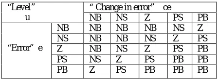
The fuzzy controller implements a rule base made of a set of IF-THEN type of rules. These rules were determined heuristically based on the knowledge of the plant. An example of IF THEN rules is the following
IF e is negative big (NB) and ce is negative big (NB) THEN u is Negative big (NB)
This rule quantifies the situation where the spherical tank system is far to minimum level to maximum level hence the control valve needed to open from 100% to 0% so that it control the particular operating point of the liquid level system. The resulting rule table is shown in the Table 1.
TABLE I.RULE BASE FOR THE FUZZY CONTROLLER
Here min-max inference engine is selected, utilizes minimum for the AND operator and maximum for the OR operator. The end of each rule, introduced by THEN, is also done by minimum. The final
“Level” u
“ Change in error” ce
NB NS Z PS PB
“Error” e
NB NB NB NB NS Z
NS NB NB NS Z PS
Z NB NS Z PS PB
PS NS Z PS PB PB
ISSN: 2231-5381
http://www.ijettjournal.org
Page 4461conclusion for the active rules is obtained by the maximum of the considered fuzzy sets. To obtain the crisp output, the centre of gravity (COG) defuzzification method is used. This crisp value is the resulting controller output.
B. Adaptive Fuzzy Control
In this section, design and development of a FMRLC, which will adaptively tune on-line the centers of the output membership functions of the fuzzy controller determined earlier.
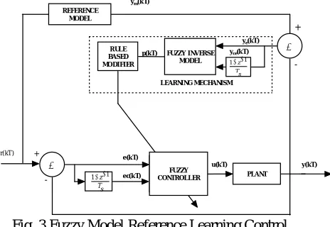
Fig. 3Fuzzy Model Reference Learning Control
Fig. 3. shows the FMRLC as applied to the spherical
tank level system. The FMRLC uses a (learning
mechanism that emphasizes
1) observes data from a fuzzy control system (i.e.
r(kT) and y(kT))
2) Characterizes its current performance, and 3) Automatically synthesizes and/or adjusts the fuzzy controller using rule base modifier so that some pre-specified performance objectives are satisfied.
In general, the reference model, which
characterizes the desired performance of the system, can take any form (linear or nonlinear equations, transfer functions, numerical values etc.). In the case of the level process reference model is shown in the fig. 3.
An additional fuzzy system is developed
called “fuzzy inverse model” which adjusts the
centers of the output membership functions of the fuzzy controller, which still controls the process, This fuzzy system acts like a second controller, which updates the rule base of the fuzzy controller by acting upon the output variable (its membership functions centers). The output of the inverse fuzzy
model is an adaptation factor p(kT) which is used by
the rule base modifier to adjust the centers of the output membership functions of the fuzzy controller.
The adaptation is stopped when p(kT) gets very small
and the changes made to the rule base are no longer
significant. The fuzzy controller used by the FMRLC structure is the same as the one developed in the previous section.
The fuzzy inverse model has a similar structure to that
of the controller (the same rule base, membership functions, inference engine, fuzzification and defuzzification interfaces. See section 3.1).
The inputs of the fuzzy inverse model are
ye(kT) = ym(kT) – y(kT) (10)
yc(kT) = ( ye(kT) – ye(KT-T) ) / T (11)
and the output variable is the adaptation factor p(kT).
The rule base modifier adjusts the centers of the
output membership functions in two stages
1) the active set of rules for the fuzzy controller at time (k-1)T is first determined
(12)
The pair (i, j) will determine the activated rule. We denoted by i and j the i-th, respectively the j-th membership function for the input fuzzy variables error and change in error.
2) the centers of the output membership
functions, which were found in the active set of rules determined earlier, are adjusted. The centers of these membership functions (bl) at time kT will have the following value
b (kT ) =b (kT- T) +p(kT) (13)
We denoted by l the consequence of the rule
introduced by the pair (i, j).
The centers of the output membership functions, which are not found in the active set of rules
(i, j), will not be updated. This ensures that only
those rules that actually contributed to the current output y(kT) were modified. We can easily notice that only local changes are made to the controller’s rule base.
For better learning control a larger number of output membership functions (a separate one for each input combination) would be required. This way a larger memory would be available to store
Information. Since the inverse model updates only the output centers of the rules which apply at that time instant and does not change the outcome of the other rules, a larger number of output membership functions would mean a better capacity to map different working the adjustments it made in the past for a wider range of specific conditions. This represents an advantage for this method since time consuming re-learning is avoided. At the same time this is one of the characteristics that differences learning control from the more conventional adaptive control.
FUZZY
CONTROLLER PLANT
FUZZY INVERSE MODEL RULE
BASED MODIFIER REFERENCE
MODEL
FUZZY CONTROLLER
-+
+
-LEARNING MECHANISM
r(kT)
e (k T)
e c(k T)
u(k T) ym(k T)
y(kT) ye(kT)
yce(k T) p(kT)
s T z1 1
s T
ISSN: 2231-5381
http://www.ijettjournal.org
Page 4462
N
1 i
2 ) i
α
i (t N
1
i N
1 2 ) i (e N 1 MSE
jk
β
1) i(k
α
1 k
1
i ijk
w k
F jk
α
k g k l k x 1 k
x
IV. NEURAL NETWORK BASED IMC
The way in which the neurons of a neural network are organised is intimately linked with the learning algorithm used to train the network. Learning algorithm used in the design of the neural networks as being structured. Feed forward neural network distinguishes itself by the presence of one or more hidden layers whose computation nodes are correspondingly called hidden neurons. The function of the hidden neurons is to intervene between the external inputs and the network output in some useful manner. Artificial neural networks (ANN) are trained by adjusting these input weights, so that the calculated outputs may be approximated by the desired values.The output from a given neuron is calculated by applying a transfer function to a weighted summation of its input to give an output, which can serve as input to other neurons as follows.
(14)
The model fitting parameters wijk are the connection
weights. The nonlinear activation transfer functions Fk. The training process requires a proper set of data
i.e., input (I1) and target output (ti). During training
the weights and biases of the network are iteratively adjusted to minimize the network performance function. The typical performance function that is used for training feed forward neural networks is the network Mean Squares Errors (MSE).
(15)
There are many different types of neural networks, differing by their network topology and/or learning algorithm. In this paper the back propagation learning algorithm,which is a multilayer feed forward network with hidden layers between the input and output. The simplest implementation of back propagation learning is the network weights and biases updates in the direction of the negative gradient that the performance function decreases most rapidly. An iteration of this algorithm can be written as follows.
(16) There are various back propagation algorithms such as Scaled Conjugate Gradient (SCG), Levenberg-Marquardt (LM) and Resilient back Propagation (RP). Among these LM is the fastest training algorithm for networks of moderate size and it has the memory reduction feature to be used when the training set is large.
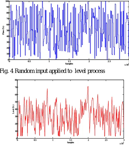
A. Generation of input-output data
By changing the flow rate as random number sequence is given as input to the spherical tank liquid level system as shown in Figure.4 and the corresponding output is obtained as shown in Fig. 5. The identification data set, containing N = 30000 samples with sampling time of 1 sec.
Fig. 4 Random input applied to level process
Fig. 5 Output data of level process by applying random input
B. Forward neural model of level process
The neural network approach is trained to represent the forward dynamics of the level system . The network is trained using delayed outputs and current input. The Activation function for the hidden layer is tansigmoidal, while for the output layer linear function is selected and they are bipolar in nature. The block diagram of forward neural network model is shown in Figure.6. The Levenberg Marquardt (LM) learning algorithm does the correct choice of the weight.
h(k)
( ) h k
Fig. 6 Block diagram of forward neural model
0 0.5 1 1.5 2 2.5 3
x 104 0
10 20 30 40 50 60 70 80 90 100
Samples
F
lo
w
(
%
)
0 0.5 1 1.5 2 2.5 3
x 104 0
10 20 30 40 50 60 70 80
Samples
L
e
v
el
(
%
ISSN: 2231-5381
http://www.ijettjournal.org
Page 44631) Training and Model Validation Of Forward
Neural Model: The data set used for training is
sufficiently rich to ensure the stable operation, since no additional learning takes place after training. During training the NN learns the forward of the level system dynamics by fitting the input-output data pairs. This is achieved by using the LM algorithm. The simulated forward model output is shown in fig. 7. It is observed from Figure.6. That forward model output exactly matches with output of the actual process. Hence, the neural network has the ability to model forward dynamics of the level system model, which can be used for developing the model based controllers.
Fig. 7 Response of forward neural model and Actual output
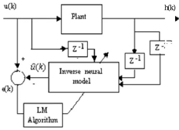
C. Direct Inverse Neural Model Of Level Process
The neural network approach is also trained
to capture the inverse dynamics of the level process model,. The network is trained using delayed sample of outputs and delayed input of level process model. The Activation function for hidden layer and output layer are bipolar tansigmoidal and bipolar pure linear are used to give the desired output, which is input signal for the level process model. The block diagram of direct inverse neural model is shown in Fig. 8.
h(k)
Fig. 8 Block diagram of inverse neural model
1) Training and Model Validation of Inverse Neural
Model: During training the NN learns the inverse of
the level system model, by fitting the input-output
data pairs. This is achieved by using the LM algorithm. It is clear from Fig. 9. That the inverse model output exactly matches with input of the actual model. Hence the neural network has the ability to model inverse, which can be used for developing
Model-based controllers.
. Fig. 9 Response of inverse neural model and actual input model
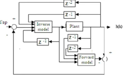
D. Design Of Neural Internal Model Controller
The Internal Model Control (IMC)
philosophy relies on the Internal Model Principle, which states that control can be achieved only if the control system encapsulates, either implicitly or explicitly, some representation of the process to be controlled. In particular, if the control scheme has been developed based on an exact model of the process, then perfect control is theoretically possible. In practice, however, process-model mismatch is common; the process model may not be invertible and the system is often affected by unknown disturbances. The open loop control arrangement will not be able to maintain output at set point. Nevertheless, it forms the basis for the development of a control strategy that has the potential to achieve perfect control. This strategy is called as Internal Model Control.The neural internal model control approach is similar to the direct inverse control approach above except for two additions. First is the addition of the forward model placed in parallel with the plant, to cater for plant or model mismatches and second is that the error between the plant output and the neural net forward model is subtracted from the set point before being fed into the inverse model. The other data fed to the inverse model is similar to the direct method. A filter can be introduced prior to the controller in this approach to incorporate robustness in the feedback system, especially where it is difficult to get exact inverse models. The neural internal model controller is shown in Fig.10.
V. RESULTS AND DISCUSSION
In this section, the simulation results for Spherical tank level system are presented to illustrate the performance of the FMRLC control algorithm.
0 0.5 1 1.5 2 2.5 3
x 104 0
10 20 30 40 50 60 70 80
Samples
L
ev
el
(
%
)
Actual model nn-forward model
0 0.5 1 1.5 2 2.5 3
x 104 0
20 40 60 80 100 120
Samples
L
e
v
el
(
%
)
ISSN: 2231-5381
http://www.ijettjournal.org
Page 4464The differential equation is derived in the section 2 are considered for this simulation study. Here, simulations are analyzed in two cases. Initially, the spherical tank is maintained at 40 % of its maximum
h(k)
Fig. 10 Block diagram of internal model control
level and a 5% step signal is applied to the process with FMRLC control algorithm and the responses are recorded in Fig. 11. Similarly, a same procedure is applied to NNIMC and ZNPI for the comparative analysis. The performance indices interms of ISE and IAE are calculated and summarized in the table 2. In order to validate the FMRLC algorithm, the different operating points (50% and 60 %) are also carried out and output responses are recorded in the fig. 12. and fig. 13. and their performance indices are given in the same table2.To analyze the FMRLC controller for the both the cases, a performance analysis in terms of ISE, IAE is made and their values are tabulated in Table 2 and Table 3
TABLE 2.PERFORMANCE INDEX FOR SERVO RESPONSE
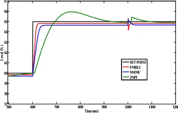
Secondly, a load disturbance is applied to the FMRLC algorithm under the same operating points and responses are traced in Fig. 14. to fig. 16. In the case of servo regulatory, the process is maintained at 40 % of its maximum level and 5% step signal is applied to the process and the disturbance is given at new steady state level (10% of given step change).
The performance indices for all the three controllers are computed and tabulated in the table 3. Also the different operating points (50% and 60 %) are also carried out and their performances indices
are summarized in the same table 3. It is observed that, the FMRLC algorithm gives an excellent performance than the other two.
TABLE 3. PERFORMANCE INDEX FOR SERVO REGULATORY RESPONSE
FMRLC NNIMC ZNPI ISE IAE ISE IAE ISE IAE
40% 133.9 92.88 182.5 102.8 674.1 331.6
50% 146.5 105.5 210.6 179.8 696.3 344.5
60% 173 149.4 324.9 278 659.8 330.6
From the table 2 and 3, it is observed that FMRLC control algorithm provides minimum error values in the servo and servo regulatory cases than the other control strategies
VI. CONCLUSION
This paper, a Fuzzy Model Reference Learning Control (FMRLC) is applied in to a non linear spherical tank system. Simulation runs are carried out by considering the FMRLC algorithm, NNIMC and conventional ZN PI-mode in a closed loop. The results clearly indicate that the incorporation of FMRLC in the control loop in spherical tank system provides a superior tracking performance than the NNIMC and conventional PI mode.
Fig. 11 Servo Response of spherical tank at 40% operation point
Fig. 12 Servo Response of spherical tank at 50% operation point
500 550 600 650 700 750 800 850 900 950 1000
37 38 39 40 41 42 43 44 45 46
Time (sec)
L
e
v
el
(
%
)
SET POINT FMRLC NNIMC ZNPI
500 550 600 650 700 750 800 850 900 950 1000
48 49 50 51 52 53 54 55 56
Time (sec)
L
e
v
el
(
%
)
SET POINT FMRLC NNIMC ZNPI
FMRLC NNIMC ZNPI ISE IAE ISE IAE ISE IAE
40% 124.2 89.48 182.3 88.32 697.2 319.5
50% 143.3 94.59 206.4 159.3 756.1 340.9
ISSN: 2231-5381
http://www.ijettjournal.org
Page 4465Fig. 13 Servo Response of spherical tank at 60% operation point
Fig. 14 Regulatory Response of Spherical tank at 40% operating point
Fig. 15 Regulatory Response of Spherical tank at 50% operating point
Fig. 16 Regulatory Response of Spherical tank at 60% operating point
REFERENCE
[1] Anandanatarajan and M.Chidambaram.”Experimental evaluation of a controller using variable tansformation on a hemi-spherical tank level process”, Proceedings of National Conference NCPICD , pp. 195-200,2005.
[2] Ya-Gang Wang, Hui-He Shao, “Optimal tuning for PIcontroller”, Automatica, vol.36, pp.147-152, 2000.
[3] T.J.Procyk, H.Mamdani, “A Linguistic self
Organizing process controller”, Automatica,vol. 15, pp.15-30, 1979.
[4] K.L.Tang, R.J. Mulholland, “Comparing fuzzy logic with classical controller design” , IEEE Transaction on systems, Manan cybernetics ,vol.17 , pp.1085-1087, 1987
[5] Isabelle Rivals. “Nonlinear internal model control using neural networks application to processes with delay and design issues”,IEEE Transaction on Neural Networks,Vol.11, No.1, pp. 80-90, Jan 2000.
[6] Hunt K J.. “Neural networks for nonlinear internal model control”,IEE.Pro-D, Vol.138, No.5, pp. 431-438, May 1991.
[7] R.Boukezzoula, S.galichet and L.Foulloy. “Nonlinear internal model control: application of inverse model based fuzzy control”,IEEE Trans.Fuzzy System, Vol.11, No.6,pp. 814- 829, Dec 2003.
[8] Adrian-Vasile Duka, Stelian Emilian Oltean, Mircea “Model reference adaptive vs. learning control for the Inverted pendulum. a comparative case study” CEAI, Vol. 9, No. 3;4, pp.67-75, 2007
[9] Scott C. Brown,Kevin M. Passino,”Intelligent Control for an Acrobot”, Journal of Intelligent and Robotic Systems Vol. 18,No. 3, March 1997, pp. 209- 248.
[10] Jeffery R. Layne, Kevin M. Passino, “Fuzzy Model Reference Learning Control for Cargo Ship Steering”. IEEE Control Systems Magazine, Vol. 13, Dec. 1993, pp. 23-34.
[11] Vijayakarthick M and P K Bhaba,” Optimized Tuning of PI Controller for a Spherical Tank Level System Using New Modified Repetitive Control Strategy”, IJERD, Vol. 3, Issue 6 (September 012),P. 74-82
500 600 700 800 900 1000 1100 1200
57 58 59 60 61 62 63 64 65 66 67
Time (sec)
L
e
v
el
(
%
)
SET POINT FMRLC NNIMC ZNPI
500 550 600 650 700 750 800 850 900 950 1000
57 58 59 60 61 62 63 64 65 66 67
Time (sec)
L
ev
el
(
%
) SET POINT
FMRLC NNIMC ZNPI
500 600 700 800 900 1000 1100 1200
37 38 39 40 41 42 43 44 45 46 47
Time (%)
L
ev
el
(
%
)
SET POINT FMRLC NNIMC ZNPI
500 600 700 800 900 1000 1100 1200
47 48 49 50 51 52 53 54 55 56 57
Time (sec)
L
ev
el
(
%
)