© 2015 IJSRSET | Volume 1 | Issue 3 | Print ISSN : 2395-1990 | Online ISSN : 2394-4099 Themed Section: Engineering and Technology
Efficient Pathloss Model for determining Mobile Radio Link Design
Alor M.O
Department of Electrical/Electronic Engineering, Enugu State University of Science and Technology, ESUT, Nigeria
ABSTRACT
The focus of this paper is on efficient pathloss model for determining mobile radio link design. A fixed 3G BTS transmitter was also used to generate the data. Log-normal shadowing model was used to analyse the data. The calculated data were compared using path loss exponent and standard deviation. They were found to be within the specified range for urban area cellular radio environment like Enugu urban. The result is a provision of a link design network with an adequate coverage and quality of service.
Keywords: Efficient Pathloss Model, Radio Propagation Mechanisms, Propagation Path Loss Models, Free Space Propagation Model, Two-Ray Model, Mobile Radio
I.
INTRODUCTION
Radio wave is a type of electromagnetic radiation (these are nothing but oscillations which propagate with the velocity of light. Approx. =3×10⁸m/s) in free space.[1] Other forms of electromagnetic waves include infrared, visible light, ultra-violet, X-rays and gamma rays [2]. Mobile radio communication systems such as cordless telephone, hand held walkie talkie, cellular and pager telephones rely on the propagation of radio waves through air and space for their operation. These radio waves travel along transmission line and waveguides to and from antennas.
The mobile radio link places fundamental limitations on the performance of wireless communication system according to wireless communication [3] The antenna at a mobile terminal is very small, so obstacles and reflecting surfaces in vicinity and path of antenna have a substantial influence on the characteristics of the propagation path between the base station transmitting antenna and the mobile antenna. The transmission path between the transmitter and the receiver may vary from direct line-of-sight (LOS) to one that is heavily obstructed by buildings and topology. This is because obstacles and reflecting objects in a mobile radio environment greatly reduce the average signal strength received by a mobile system.
II.
METHODS AND MATERIAL
2. The radio propagation mechanisms
The radio propagation mechanisms which impact propagation in a mobile communication system are:
i. Reflection ii. Diffraction iii. Scattering
Mobile communication conditions operation is quit severe; the reason is that most cellular radio systems which operate in urban area operate with no direct Line-of-sight (LOS) path between the transmitter and the receiver. The presence of high building creates severe diffraction loss.
The path loss is generally the most important parameter predicted by propagation models based on the physics of reflection, diffraction and scattering.
Reflection occurs when electromagnetic waves impinges on obstacles with larger wavelength.
Diffraction therefore, remains an important phenomenon where signal transmission through buildings is virtually impossible.
Scattering occurs when objects are of dimensions that are in the order of a wavelength or less of the electromagnetic waves. Scattered waves are produced by irregular objects such as walls with rough surface, furniture, foliage etc.
2.1 Propagation path loss models
Path loss is defined as the difference in decibel between the effective transmitted power and the received power and perhaps includes the effect of antenna gains. It represents signal attenuation as a positive quantity measured in dB [4]. Some of these models are discussed in this section.
A. Free Space Propagation Model
Free space propagation environment is a region that is free of all obstacles and objects that might absorb or reflect radio frequency energy. Free space propagation model assumes an ideal propagation with an isotropic antenna radiating its energy equally in all directions to an infinite distance. If the radiating element is generating a fixed power to an ever expanding sphere, the power density on this hypothetical sphere at a distance d from the source is given by equation 1 below:
14 d2 P G d
P t t
)
Where :
Pt is the transmitted power
Gt is the transmitting antenna gain
d is distance from the source.
If a receiving antenna with gain Gr is placed at this
distance, d, the power extracted by the antenna can be calculated using equations (2)
Pr = P(d) Ae
(2) Where ,
Pr is the received power
e
A
is the effective area of an isotropic antenna
4
2
eA
(3)
(
4
)
4
2 t r t e rP
d
G
G
A
d
P
P
The free space transmission loss or propagation loss equations for Omni directional transmit and receive unity gain antennas separated by d meters is obtained as:
)
5
(
4
2
d
G
G
P
P
t t t r
For Omni directional and unity gain antenna, free space path loss is given in equation (6) which is also known as Friis equation.
)
6
(
4
2
d
P
P
t r
)
7
(
4
2
f d
c
P
P
t r
In terms of pathloss in dB,
r tP
P
dB
Pl
[
]
10
log
Where,
PL is Path loss in [dB]
Pt is the transmitted power
Pr is the received power
The free space path loss equation is now:
PL[dB] = 32.44 log f [MHz] log d [km]
(8)
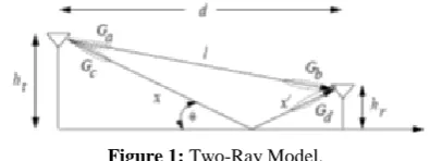
B. Two-Ray Model
The two-ray model is used when a single ground reflection dominates the multipath effect, as illustrated in Figure1. The received signal consists of two components: the LOS component or ray, which is just the transmitted signal propagating through free space, and a reflected component or ray, which is the transmitted signal reflected off the ground.
C. Mobile Radio Link
Communication engineers are generally concerned with the application of two main radio channel links. These channel links are the mobile radio link parameters and time dispersion nature of the channel.
The mobile radio link parameters consist of the path loss exponents (n) or path loss rate and the standard deviation (
) about its mean value. The path loss exponent indicates the rate at which propagation (path) loss increases with distance, while the standard deviation accounts for the random shadowing effects which occur over a large number of measurement locations which have same transmitter-receiver separation, but have different levels of clutter on the propagation path [5].The emphasis of this research is on the determination of mobile radio link design for a given propagation environment using path loss model. These parameters are used in link budget design to determine fundamental quantities such as transmit power requirements, coverage areas, battery life and the analysis of path losses in any mobile radio environment.
The time dispersive parameters of a multipath channel are the mean excess delay, rms delay spread and the maximum excess delay spread [6]. The time dispersive nature of the channel determines the maximum data rate that can be transmitted without equalization.
2.2 Practical link budget determination using the path loss models
Most radio propagation models are derived using a combination of analytical and empirical methods. The empirical approach is based on fitting curves or analytical expressions that recreate a set of measured data. This has the advantage of implicitly taking into account all propagation factors, both known and unknown, through actual field measurements. However, the validity of empirical models at transmission frequencies or environments other than those used to derive the model can only be established by additional measured data in the new environment at the required frequency. Over time, some classical empirical models have emerged, which are now used to predict both
large-scale and medium-scale coverage for mobile communication system design. The two practical mobile radio link design techniques are:
i. The log-distance path loss model. ii. The log-normal path loss model.
(i) The log-distance path loss model
Both theoretical and measurement based propagation models indicate that the coverage received signal power decreases logarithmically with distance, whether in outdoor or indoor radio channels. The average large-scale path loss for an arbitrary transmit-receiver (T-R) separation is expressed as a function of distance by using path loss exponent (n) as
) 9 ( )
/ ( )
(d d do n PI
Or
)
10
(
)
/
log(
10
)
(
)
(
dB
PL
d
0n
d
d
0PL
Where n is the path loss exponent,
d
0 is the closed-in reference distance which is determined from measurements closed to transmitter and d is the T-R separation distance. The value of n depends on the specific propagation environment. For example if free space is 2 and when obstructions are present, n will have a larger value as shown in table 1 [7]It is important to select a close in reference distance that is appropriate for the propagation environment. In large coverage cellular systems, 1km reference distance is commonly used, whereas in microcellular systems smaller distance such as 100m is commonly used. The reference distance should always be in the far field of the antenna so that near field effect does not alter the reference path loss. The reference path loss PL(do) is
calculated using free space path loss formula given equation (1) or through field measurement at distance (do). Table 1 list path loss exponents obtained in mobile
radio environment
Table 1: Path loss exponents for different environments
Environment Path loss Exponent, n
Urban cellular/PCS 2.7 to 4.0
Shadowed urban
cellular/PCS
3 to 5
Indoor LoS 1.6 to 1.8
Obstructed Indoor 4 to 6 Obstructed in factories 2 to 3
(ii) The log-normal shadowing model
The log-distance path model does not consider the fact that the surrounding environmental clutter may be vastly different at two different locations having the same T-R separation. This leads to measured signals, which are vastly different from the average value predicted by (10).
The log-normal distribution describes the random shadowing effects which occur over a large number of measurement locations which have the same T-R separation, but have different levels of clutter on the propagation path. This phenomenon is referred to as log-normal shadowing. Log-log-normal shadowing implies that measured signal level at a specific T-R separation have a Gaussian (normal) distribution about the distance-dependent mean of equation 10 where the mean signal levels have values in dB. The standard deviation of the Gaussian distribution that describes the shadowing also in dB.
Measurements have shown that at any value of d, the path loss PL(d) at a particular location is random and distributed log-normally (normal in dB) about the mean distance dependent value. i.e.
) 11 ( )
( ]
)[
(d dB PL dB x
L
P
)
12
(
log
10
)
(
]
)[
(
0
0
n
d
d
x
d
L
P
dB
d
L
P
And,
) 13 ( ]
)[ ( ]
[ ]
)[
Pr(d dBm Pt dBm PL d dB
Where
x
is a zero-mean Gaussian distributed random variable (dB) with standard deviation
also in dB. The closed in reference distance (d0), the path loss exponent (n), and the standard deviation (
) statically describe the path loss model for an arbitrary locationhaving a specific T-R separation and this model may be used in computer simulation to provide received power levels for random locations in communication system design and analysis [8]
III.
RESULTS AND DISCUSSION
The real time measurements were conducted using CDMA 2000 1x BTS located at Headquarter opposite Teachers House Enugu as the test transmitter location. The eight radial field measurements were carried along specific separation distances for North, West and East routes.
The field measurement were carried out using 3G CDMA technology rather than the GSM because of its advantages such as higher bandwidth capacity, high-speed packet data and multipath fading reduction.
(A) Data Gathering
The field measurement were carried out using a radio propagation simulator called debug access equipment global positioning system (GPS) and simulation of free space model equation.
The GPS indicates the T-R separation distances while the debug access equipment measured received power levels at various distances away from a CDMA 2000 1xBTS.
The simulation was also done to compare the received signal levels at the eight radial distances.
4.0 System Specification
The system design for the 3G CDMA BTS at various separation distances and the received power are specified as follows:
A. Base Transceiver Station
BTS transmit power = 10w
BTS antenna gain = 20dB
B. Mobile Station (MS)
MS transmit power = 300MW
MS Sensitivity less than = 104dB
MS antenna gain = 0dB
MS transmitter carrier
Frequency = 841.25MHz
Height of MS antenna = 1.6m
Average cell radius = 5km
The distance between BTS = 9km
The eight received power measurement taken at various distances radially along North, West and East were designed as follows using (14) and (15)
4
(
14
)
log
10
)
(
2 0 2 2 0d
G
G
P
d
Pi
t t r
)
15
(
log
10
)
(
0 0
P
i
d
n
d
d
i
P
where,
d = T-R separation distance. d0 = close in reference distance
x
= zero-mean Gaussian (normal)distributed random variable (dB) with standard deviation,
(dB).From the parameter, Pt =10w
Gt =20dB = 100
Gr = 0dB = 1 d0 = 100m f = 881.25×106
= 0.34m From equation 14
2 2 20
)
100
(
4
)
34
.
0
(
1
100
10
log
10
)
(
d
Pi
)
(
d
0Pi
= 41.36dBmThen using field measurement at a close in reference
distance (d0) of 100m,
Pi
(
d
0)
= -40dBm. So, recall equation (15) and substitute,
100
log
10
40
n
d
i
P
Based on the field measurement the estimated received power for the specified distances were found using (15).
For 100m,
100
100
log
10
40
1n
P
Pi = -40 For 200m,
100
200
log
10
40
2n
P
P2 = – 40 – 3n
For 500m,
100
500
log
10
40
3n
P
P3 = – 40 – 7n For 1000m,
100
1000
log
10
40
4n
P
P4 = – 40 – 10n For 2000m,
100
2000
log
10
40
5n
P
P5 = – 40 – 13n For 3000m,
100
3000
log
10
40
6n
P
P6 = – 40 – 15n For 4000m,
100
4000
log
10
40
7n
P
P7 = – 40 – 16n
For 5000m,
100
5000
log
10
40
8n
P
P8 = – 40 – 17n
2194
6878
n
n = 3.13 3.1
The path loss exponent for the mobile radio link is 3.1
Table 3 : Received power measurement taken at various distances along North, West and East Routes
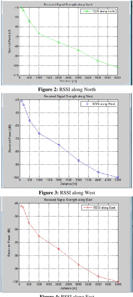
The plot of the received signal strength along the different routes is shown in Figure 2, Figure 3,Figure 4 and Figure 5
Figure 2: RSSI along North
Figure 3: RSSI along West
Figure 4: RSSI along East
IV.
CONCLUSION
Mobile radio link design using path loss model can be easily designed using parameters of base transceiver station (BTS), mobile stations (MS) and the Log-normal shadowing pathloss model. In this paper, the path loss exponent and the standard deviation due to random shadowing in Enugu urban are 3.1 and 5.65dB respectively. These Mobile radio link designs were determined using the Log-normal shadowing path loss model. The path loss exponent value shows the rate at which the pathloss increases with distance in a CDMA2000 1x. This path loss model is very good for predicting distance dependant received power in obstructed environment. The accurate qualitative understanding of the radio propagation using path loss model as a function of distance from where the signal level could be predicted is essential for reliable wireless system design.
V.
REFERENCES
[1] Michael J. Martin, (2006), “Radio frequency Physics: the
rules are changing”, IBM Canada, January 2006.
[2] Waltisch,J. et al,(2008)" A theoretical model of uhf propagation in urban environments",IEEE Transactions on Antenna and propagation pp 1788-1796
[3] Rappaport T.S.,(2006)"Wireless communication principles and practice"Pearson Education.
[4] Guptel V,et al,(2008) "Efficient pathloss prediction in mobile wireless communication Networks, proceeding of world Academy of Science, Engineering and Technology, Vol 36.
[5] Smith M.S. et al,(2000)"A new methodology for delivery pathloss model for cellular drive test data.
[6] Simon Haykins–Communication Systems-John Willy & Sons ,Fourth edition
[7] Kathryn Oliver, (2004), “Introduction to Automatic
Design of Wireless Networks”, Centre for Intelligent Network Design, Cardiff University, UK, 2004.