Modeling Approaches for Cost and Cost-Effectiveness Estimation Using Observational Data

University of Pennsylvania

ScholarlyCommons

Publicly Accessible Penn Dissertations

1-1-2016

Modeling Approaches for Cost and

Cost-Effectiveness Estimation Using Observational Data

Jiaqi Li

University of Pennsylvania, [email protected]

Follow this and additional works at:

http://repository.upenn.edu/edissertations

Part of the

Biostatistics Commons

This paper is posted at ScholarlyCommons.http://repository.upenn.edu/edissertations/1858

Recommended Citation

Li, Jiaqi, "Modeling Approaches for Cost and Cost-Effectiveness Estimation Using Observational Data" (2016).Publicly Accessible Penn Dissertations. 1858.

Modeling Approaches for Cost and Cost-Effectiveness Estimation Using

Observational Data

Abstract

The estimation of treatment effects on medical costs and cost effectiveness measures is complicated by the

need to account for non-independent censoring, skewness and the effects of confounders. In this dissertation,

we develop several cost and cost-effectiveness tools that account for these issues. Since medical costs are often

collected from observational claims data, we investigate propensity score methods such as covariate

adjustment, stratification, inverse probability weighting and doubly robust weighting. We also propose several

doubly robust estimators for common cost effectiveness measures. Lastly, we explore the role of big data tools

and machine learning algorithms in cost estimation. We show how these modern techniques can be applied to

big data manipulation, cost prediction and dimension reduction.

Degree Type

Dissertation

Degree Name

Doctor of Philosophy (PhD)

Graduate Group

Statistics

First Advisor

Nandita Mitra

Keywords

cost effectiveness, cost estimation, doubly robust, machine learning, net monetary benefit, propensity score

Subject Categories

MODELING APPROACHES FOR COST AND COST-EFFECTIVENESS ESTIMATION USING OBSERVATIONAL DATA

Jiaqi Li

A DISSERTATION

in

Epidemiology and Biostatistics

Presented to the Faculties of the University of Pennsylvania

in

Partial Fulfillment of the Requirements for the

Degree of Doctor of Philosophy

2016

Supervisor of Dissertation

Nandita Mitra, Associate Professor of Biostatistics

Graduate Group Chairperson

John H. Holmes, Professor of Medical Informatics in Epidemiology

Dissertation Committee

Scarlett Bellamy, Associate Professor of Biostatistics

Dylan Small, Professor of Statistics

Elizabeth Handorf, Assistant Research Professor at Fox Chase Cancer Center

MODELING APPROACHES FOR COST AND COST-EFFECTIVENESS ESTIMATION USING

OBSERVATIONAL DATA

c

COPYRIGHT

2016

Jiaqi Li

This work is licensed under the

Creative Commons Attribution

NonCommercial-ShareAlike 3.0

License

To view a copy of this license, visit

ACKNOWLEDGEMENT

My deepest gratitude is to my advisor, Dr. Nandita Mitra. I have been amazingly fortunate to have

an advisor who gave me the freedom to explore on my own, and at the same time the guidance

to recover when my steps faltered. Nandita has always been there since day one of my graduate

studies. The guidance I received from her made my Ph.D. purposeful and fulfilling, and I can

not imagine having a better advisor and mentor than her. Nandita taught me how to become a

researcher, to question thoughts and express ideas and I could not finish this dissertation without

her patience and support.

I would like to thank the chair of my dissertation committee Dr. Scarlett Bellamy, for her insightful

comments and constructive criticisms at different stages of my research. I would also like to thank

my committee members, Dr. Dylan Small and Dr. Justin Bekelman, who have been there since

my master thesis. They have given guidance and had patience over the years, taking their time to

carefully read and evaluate my research work. My dissertation member, co-author, and “academic

sister” Dr. Elizabeth Handorf has helped me in collaboration projects, dissertation research and

given me valuable career advice. Finally, my sincere thanks goes to all the faculty, students, staff

and alumni of the Biostatistics Department. I am extremely grateful to several faculty members,

including Dr. Mary Putt, Dr. Hongzhe Li, Dr. Benjamin French, Dr. Sharon Xie, as well as Edward

Kennedy for their engagement and practical advice throughout my Ph.D career.

Lastly, I would like to thank my husband Shiliang Cui, my parents, my family and my best friends

Miao Wang and Ayla Jiang, for the unconditional love and support during the past four years.

They all kept me going, and this journal of academic exploration would not be possible with their

ABSTRACT

MODELING APPROACHES FOR COST AND COST-EFFECTIVENESS ESTIMATION USING

OBSERVATIONAL DATA

Jiaqi Li

Nandita Mitra

The estimation of treatment effects on medical costs and cost effectiveness measures is

compli-cated by the need to account for non-independent censoring, skewness and the effects of

con-founders. In this dissertation, we develop several cost and cost-effectiveness tools that account

for these issues. Since medical costs are often collected from observational claims data, we

in-vestigate propensity score methods such as covariate adjustment, stratification, inverse probability

weighting and doubly robust weighting. We also propose several doubly robust estimators for

com-mon cost effectiveness measures. Lastly, we explore the role of big data tools and machine learning

algorithms in cost estimation. We show how these modern techniques can be applied to big data

TABLE OF CONTENTS

ACKNOWLEDGEMENT . . . iii

ABSTRACT . . . iv

LIST OF TABLES . . . vii

LIST OF ILLUSTRATIONS . . . viii

CHAPTER 1 : INTRODUCTION . . . 1

1.1 Background . . . 1

1.2 Novel developments . . . 6

CHAPTER 2 : PROPENSITY SCORE AND DOUBLY ROBUST METHODS FOR ESTIMATING THE EFFECT OF TREATMENT ON CENSORED COST . . . 8

2.1 Introduction . . . 8

2.2 Cost estimation - existing methods . . . 10

2.3 Propensity score approaches . . . 12

2.4 Doubly Robust Estimation . . . 17

2.5 Super-Learning . . . 19

2.6 Simulation studies . . . 20

2.7 Costs of Bladder Cancer Therapies . . . 25

2.8 Discussion . . . 28

2.9 Acknowledgment . . . 29

CHAPTER 3 : DOUBLY ROBUST METHODS FOR COST-EFFECTIVENESS ESTIMATION FROM OBSERVATIONAL DATA . . . 30

3.1 Introduction . . . 30

3.2 Common CE measures . . . 32

3.3 CE estimation . . . 33

3.4 Simulation studies . . . 38

3.6 Summary . . . 44

CHAPTER 4 : MODERNSTATISTICAL ANDMACHINELEARNINGAPPROACHES FORHEALTH CARECOSTESTIMATION FROMBIGDATA . . . 47

4.1 Introduction . . . 47

4.2 Big data storage and manipulation . . . 49

4.3 Cost prediction . . . 51

4.4 Dimension reduction / variable selection . . . 60

4.5 Discussion . . . 62

CHAPTER 5 : DISCUSSION. . . 63

5.1 Conclusion . . . 63

5.2 Future Directions . . . 64

APPENDICES . . . 65

LIST OF TABLES

TABLE 2.1 : %Bias, coverage and relative efficiency for estimated treatment effect on cost 23 TABLE 2.2 : %Bias, coverage and relative efficiency for estimated treatment effect on

cost under different PS estimation methods . . . 24

TABLE 2.3 : Estimated mean cost difference for bladder preserving therapy and radical cyccwetomy . . . 27

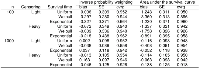
TABLE 3.1 : E(T) simulation results: inverse probability weighting vs. area under the survival curve . . . 39

TABLE 3.2 : Simulation set up: four cost distributions . . . 40

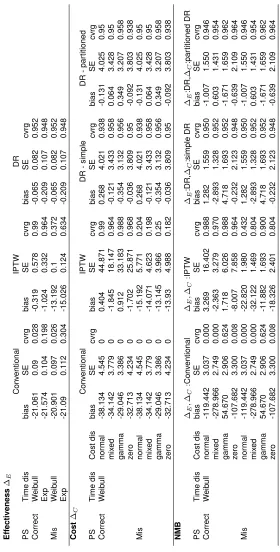
TABLE 3.3 : Simulation results: cost, effectiveness and NMB estimation . . . 42

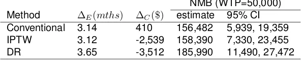
TABLE 3.4 : CE analysis of CT vs. X-ray (reference) for lung cancer surveillance . . . 44

LIST OF ILLUSTRATIONS

FIGURE 2.1 : Density of uncensored total costs in bladder cancer cohort . . . 26

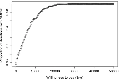
FIGURE 3.1 : CE acceptability curve of CT vs. X-ray . . . 45

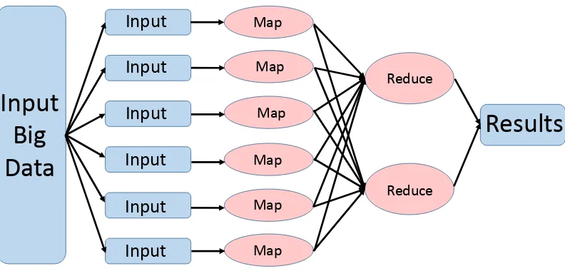
FIGURE 4.1 : MapReduce paradigm . . . 50

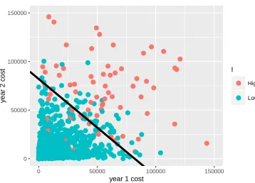
FIGURE 4.2 : Separating year 3 high and low cost patients . . . 55

CHAPTER 1

I

Proper medical cost and cost-effectiveness estimation is critical for health economics evaluation

and decision-making. We are often most interested in the effect of a new treatment on cost and

cost-effectiveness compared to the existing treatment. The gold standard for estimating the

treat-ment effect is a randomized controlled trial. However, it is often not feasible or ethical to carry

out trials just for the purpose of collecting medical cost data. Hence, we need to obtain cost and

cost-effectiveness measures from observational sources.

1.1. Background

The development of methods for the analysis of cost and cost-effectiveness data has been of

inter-est to many statisticians and health economists. In this section, we review several popular methods

that handle the unique features of cost data, including informative censoring, heteroscadasticity,

skewness and zero costs. We also provide a review of common cost effectiveness measures. Since

observational data play an important role in cost and cost-effectiveness estimation, we review

sev-eral common propensity score models that handle data from observational sources. Lastly, we give

some background on big data and machine learning tools that could be applied to cost estimation.

1.1.1. Background about cost estimations

Medical costs often have very different distributions depending on such the disease and treatment

setting. To handle distributional skewness and structural zeros, economists and statisticians have

developed two broadly categorized methods:, single equation and multiple equation models.

Sin-gle equation methods include ordinary least squares regression, generalized linear regression,

parametric models (e.g. Weibull, Gamma) with different transformations (e.g. log, Box-Cox) and

different variance functions. Some (Lumley et al., 2002) argue that with a large enough sample size

(n > 500), linear regression and t-tests are appropriate for analysis of highly skewed outcomes, including costs. Mihaylova et al. (2011) carried out a study to review some popular methods for

analyzing cost data, and recommended using a simple method such as linear regression that

and advise against ignoring skewness of cost data because variance estimates based on normal

approximations may be biased.

Historically, the natural logarithm of costs in ordinary least squares regression (OLS) or generalized

linear model (GLM) with log link have been used. However, Manning and Mullahy (2001) found OLS

estimators can be biased under heteroscadasticity. Even though GLM estimators are consistent,

they can yield imprecise estimates if the log-scale error is heavy-tailed. Manning, Basu, and

Mul-lahy (2005) evaluated OLS, OLS for log cost, standard gamma model and exponential with a log

link, and the Weibull model and found that a generalized gamma distribution was the most robust.

Several GLM based estimators have also been proposed. For example, Basu and Rathouz (2005)

proposed GLM using box cox transformation and parametric models for the variance as a function

of the mean. Others have suggested using median regression since the median is less sensitive to

skewness and outliers. Bang and Tsiatis (2002); Ying, Jung, and Wei (1995) extended median

re-gression to incorporate simple weights to handle censored cost data. Dodd et al. (2006) compared

normal and bootstrapped multiple linear regression, median regression, gamma model with the log

link and OLS of log costs. They found that GLM with log link and gamma variance provided the

best fit. Lastly, Basu, Manning, and Mullahy (2004) conducted a similar comparison and applied

popular medical cost models to different cost data structures and arrived at the same conclusion

-GLM with log link and gamma variance is the most robust model.

In addition, multiple equation models have focused on different components of costs such as zero

and non-zero costs, and inpatient and outpatient billings (Duan et al., 1983; Leung and Yu, 1996).

The rationale behind these multiple equation models are that costs accrued at different times of a

patient’s history follow different distributions and thus should be modeled differently.

One of the biggest issues present in most cost data is informative censoring due to the lack of

a common rate of cost accrual over time among patients. To handle non-ignorable censoring, the

popular approaches are either weighting-based (Bang and Tsiatis, 2000; Lin et al., 1997) or survival

model based. The latter is less popular; Etzioni et al. (1999) demonstrated that standard survival

techniques yield biased estimates. Lin et al. (1997) proposed a non-parametric approach that splits

the time period into small intervals and weights mean costs from each interval by survival

proba-bilities estimated from the Kaplan-Meier curve. Lin’s method is only consistent if the partitions are

(Bang and Tsiatis, 2000) proposed two popular methods: simple weighted and partitioned

estima-tors, to estimate mean medical cost. The simple weighted method averages subjects with complete

cost information weighted by the probability of not being censored. The The partitioned estimator

builds on the same weighting idea but makes use of cost history information and is hence more

efficient. Many (Raikou and McGuire, 2004; Zhao, Cheng, and Bang, 2011; Zhao et al., 2007) have

studied the properties of these two popular methods. Baser et al. (2004); Lin (2000, 2003)

subse-quently extended these methods to regression of censored cost. Recent work (Basu and Manning,

2010; Tian and Huang, 2007) has focused on two part models to accommodate significant zeroes,

end of life cost and skewness properties of medical cost data.

1.1.2. Background : cost effectiveness estimation

Cost effectiveness (CE) analysis is often used to evaluate the merits of a new health-care

inter-vention (treatment,Z = 1) compared to an existing one (control, Z = 0). CE measures integrate estimates of costs and effectiveness in a single statistic derived from two components:∆Eand∆C where∆E =EffectivenessZ=1−EffectivenessZ=0and∆C=CostZ=1−CostZ=0.

One common approach to combine the cost and effect outcomes to form Incremental Cost-

Ef-fectiveness Ratio (ICER). However, a major limitation of the ICER is its discontinuity when the

denominator∆Eapproaches zero. Another issue is that ICER often has an unstable interpretation; when the∆E is positive and∆C is negative, ICER has a different interpretation than when∆C is positive and∆E is negative. In addition, estimating the variance of ICER is problematic due to the acknowledged statistical problems associated with ratio statistics. Non-parametric bootstrapping,

Fieller’s theorem and Bayesian approaches (Heitjan, Moskowitz, and Whang, 1999; Polsky et al.,

1997; Willan and O’Brien, 1996) can be applied to estimate the variance of ICER.

Recently, health economists have advocated the use of the Net Monetary Benefit (NMB): NMB(λ) =

λ∆E−∆C. NMB is a linear combination of∆C and∆Eand measures the excess benefit given a fixed level ofλ. λ is defined as willingness to pay (WTP), which is the maximal monetary value

decision-makers are willing to pay for a unit of ∆E. Typically, λ measures the dollar amount one is willing to pay for one year of additional life. The NMB does not suffer from the

singular-ity problem that the ICER does. Moreover, the interpretation of NMB is straightforward: a positive

treat-ment is less cost-effective compared to the control. It is also easy to estimate its variance as

var(NMB(λ)) =λ2_var(∆

E) +var(∆C)−2λcov(∆E,∆C).

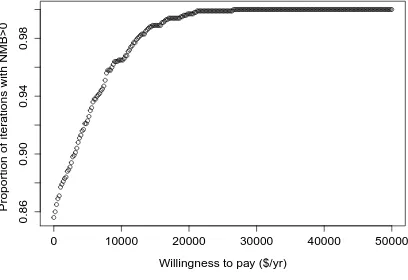
A CE acceptability curve builds on the idea underlying the NMB and displays the probability that

the treatment is cost-effective (NMB>0) compared with the control for a range ofλvalues. To plot the CE acceptability curve, we use bootstrapping to estimateP r(λ∆E−∆C >0). In practice, we simply count the proportion of bootstrapped samples that yieldsλ∆E−∆C > 0 for a range ofλ values.

Similar to cost analysis, CE estimation needs to account for informative censoring in cost data.

Willan et al. (2002) proposed NMB and ICER estimation methods accounting for censoring in cost

data in the setting of randomized trials. A similar approach was taken to extend to developing a

linear regression method that accommodates censored outcomes (Willan, Lin, and Manca, 2005).

1.1.3. Background: propensity score methods

Heath care cost information are often collected from observational claims data, thus one must be

careful when dealing with potential confounding. The propensity score (PS), first introduced by

Rosenbaum and Rubin (1983) is commonly employed to adjusted for confounding in observational

studies (Austin, 2011). Propensity scores are often used in covariate adjustment, matching,

strat-ification, and weighting (Lunceford and Davidian, 2004; Rosenbaum, 1987). Covariate adjustment

on PS is easy to use but assumes that the relationship between the propensity score and the

out-come has been correctly modeled (Austin and Mamdani, 2006), which could be a challenge in cost

estimation since there is no one-size-fits-all cost model. Rosenbaum (1987) first introduced inverse

probability of treatment weighting (IPTW) while Lunceford and Davidian (2004) presents two other

types of weights. Robins, Rotnitzky, and Zhao (1994) provided the theory behind a broader class

of weighted estimators. Matching is commonly used in practice where we match subjects in

treat-ment and control groups according to their estimated propensity scores. Stratification based on the

quintiles of the PS eliminates approximately 90% of bias due to measured confounders (Cochran,

1968; Rubin and Rosenbaum, 1984). Many have compared the relative performance of these

var-ious methods (Austin, Grootendorst, and Anderson, 2007; Austin and Mamdani, 2006; Lunceford

and Davidian, 2004). As Rubin (2004) notes, covariate adjustment using PS and IPTW are more

Recently, a new PS method, doubly robust (DR) estimation based on Robins, Rotnitzky, and Zhao

(1994) has become popular. It has the smallest large sample variance among the class of weighted

estimators. DR estimation combines outcome regression (regression model) with weighting by PS

(PS model) such that it is robust to misspecification of one (but not both) of these models (Bang

and Robins, 2005; Tsiatis and Davidian, 2007). The doubly robust property is appealing but can

result in biased estimates if both the outcome model and PS model are misspecified (Funk et al.,

2011).

1.1.4. Background : big data and machine learning methods

With the recent availability of big data, the role of machine learning in economics has become

increasingly important (Varian, 2014). Traditionally cost data have been be stored and manipulated

on spreadsheets or by a Structured Query Language (SQL). However, these tools are inadequate

for massive data which require special programing paradigms. . Some popular big data storage

and manipulation algorithms include Hadoop File Distribution System (Lam, 2010; Shvachko et al.,

2010; Venner, 2009) and MapReduce (Dean and Ghemawat, 2008).

Cost prediction has been of great interest to health economists (Folland, Goodman, Stano, et al.,

2007). Traditionally, parametric models have been used for cost prediction. In recent studies,

ma-chine learning non-parametric algorithms has been shown to have better predictive abilities (Kim,

An, and Kang, 2004; Sushmita et al., 2015). Bertsimas et al. (2008) compared the performance

of classification trees, clustering, and traditional models for cost bucket estimation, and found that

data-mining methods provide more accurate predictions. Popular machine learning prediction

algo-rithms include classification and regression trees, random forests, support vector machines,

boost-ing and Bayesian additive regression trees.

In addition, variable selection can be challenging in cost estimation models. We often have many

potential predictors that may need to be narrowed down for model building. Traditionally,

re-searchers use stepwise regression and model complexity measures such as the Akaike information

criterion (AIC) and Bayesian information criterion (BIC) to select important variables. With the rise

of big data, we see more and more large datasets with numerous potential predictors where modern

dimension reduction methods may serve as important tools in estimating cost. Popular dimension

modeling with machine learning.

1.2. Novel developments

In this dissertation, we develop statistical methods for cost and cost-effectiveness estimation from

observational data. The dissertation consist of three parts. In Chapter 2, we investigate

propen-sity score (PS) based methods such as covariate adjustment, stratification and inverse probability

weighting taking into account informative censoring of the cost outcome. We compare these more

commonly used methods to doubly robust weighting. We then use a machine learning approach

called Super-Learner (SL) to 1) choose among conventional regression models to estimate mean

models in the DR approach and 2) choose among various covariate specifications for PS

estima-tion. Our simulation studies show that when the PS model is correctly specified, weighting and

DR perform well. When the PS model is misspecified, the combined approach of DR with Super

Learner can still provide unbiased estimates. SL is especially useful when the underlying cost

dis-tribution comes from a mixture of different disdis-tributions or when the true PS model is unknown. We

apply these approaches to a cost analysis of two bladder cancer treatments, cystectomy versus

bladder preservation therapy, using SEER-Medicare data.

In Chapter 3, we propose using separate doubly robust (DR) methods based on propensity scores

for estimating CE with and without incorporating cost history and show they are unbiased. We then

use cross validation to choose among popular cost models to estimate regression parameters in

the DR approach and to choose among various parametric and non-parametric propensity score

models. Our simulation studies demonstrate that the proposed DR models perform well even under

misspecification of either the PS model or the outcome model. We apply these approaches to a

cost-effectiveness analysis of two competing lung cancer surveillance procedures, CT versus chest

X-ray, using SEER-Medicare data.

In Chapter 4, we review and explore the use of big data and machine learning techniques in health

care cost estimation. Specifically, we look at three areas: big data manipulation, cost prediction and

variable dimension reduction. Massive health care cost data calls for the use of big data storage

and manipulation algorithms like Hadoop and MapReduce. Traditionally, the focus of cost

predic-tion has been on how to come up with the best parametric model to predict cost. With the rise

classification and regression trees, random forest, Bayesian adaptive regression trees, and support

vector machines. Moreover, popular dimension reduction tools such as LASSO and principle

com-ponents analysis combine the strengths of statistical modeling with machine learning, and allow

us to identify important covariates affecting one’s health care cost and to build parsimonious cost

models. We demonstrate the use of these state-of-the-art big data and machine learning models

CHAPTER 2

P

EFFECT OF TREATMENT ON CENSORED COST

2.1. Introduction

Proper medical cost estimation is imperative to health economics evaluation and decision-making.

Policy makers are often most interested in the average effect treatment effect (ATE) on total costs.

Since medical costs are often collected from claims data which are susceptible to confounding,

appropriate estimation of the ATE from observational data demands attention. These methods

must also account for other complicating features of cost data including informative censoring and

skewness.

The primary focus of earlier studies of cost estimation has been on methods for dealing with their

distributional skewness. Historically, researchers have used natural logarithm transformed costs in

ordinary least square regression (OLS) or used generalized linear models (GLM) with a log link.

However, Manning and Mullahy Manning and Mullahy (2001) showed that OLS estimators can

be biased under heteroscadasticity and GLM estimators can yield imprecise estimates if the

log-scale error is heavy-tailed. Others have suggested using median regression since the median is

less sensitive to skewness and outliers (Manning, Basu, and Mullahy, 2005). Several studies (Basu,

Manning, and Mullahy, 2004; Basu and Rathouz, 2005; Dodd et al., 2006) have evaluated additional

approaches such as OLS, OLS for log cost, standard gamma, standard GLM, generalized gamma,

median regression, exponential models with log link, and the weibull model. Dodd et al. (2006)

found the generalized gamma model to be the most robust cost model. Recent works (Basu and

Manning, 2010; Tian and Huang, 2007) have focused on two part models and Bayesian approaches

to accommodate structural zeros and end of life costs.

An important feature of medical costs is censoring, which often occurs if the study terminates after a

fixed follow-up period. Even though survival time is non-informatively censored due to end-of-study

censoring, cost is not. Censoring in cost is informative since the rate of cost accrual over time

of mean cost by partitioning study period into subintervals and assuming censoring occurs only

at the boundaries of these subintervals. Bang and Tsiatis (2000) improved on Lin et al.’s work

and proposed two popular methods: the simple weighted method and the partitioned method, to

estimate mean medical cost under informative censoring. The simple weighted method averages

subjects with complete cost information weighted by the inverse of the probability of not being

censored. The partitioned estimator builds on the same weighting idea but also makes use of cost

history information and is therefore more efficient. Properties of these methods have been widely

studied (Raikou and McGuire, 2004; Zhao, Cheng, and Bang, 2011; Zhao et al., 2007) . Baser

et al. (2004); Lin (2000, 2003) have since extended these methods to linear regression and general

linear models to incorporate the effect of covariates. Several studies (Bang and Tsiatis, 2002; Ying,

Jung, and Wei, 1995) have also applied these techniques to median regression to handle censored

cost data.

Heath care cost information is often collected from observational sources, such as Medicare,

ne-cessitating the need to adjust for potential confounders. The propensity score (PS), first introduced

by Rosenbaum and Rubin (1983) is commonly employed to adjust for confounding in observational

studies (Austin, 2011). Propensity scores are often used in covariate adjustment, matching,

strat-ification and weighting (Lunceford and Davidian, 2004; Rosenbaum, 1987). Covariate adjustment

of the PS is easily implemented but is sensitive to the assumption that the relationship between

the propensity score and the outcome has been correctly modeled (Austin and Mamdani, 2006).

Stratification based on PS is also often used as it greatly simplifies implementation over standard

methods;Rubin and Rosenbaum (1984) demonstrated that stratification based on the quintiles of

the PS eliminates approximately 90% of bias due to measured confounders. More recently, inverse

probability of treatment weighting (IPTW) (Rosenbaum, 1987) has become the method of choice.

The normalized version of IPTW has been proposed (Busso, DiNardo, and McCrary, 2014; Hirano,

Imbens, and Ridder, 2003) which belongs to a broader class of weighted estimators described by

Robins, Rotnitzky, and Zhao (1994). Several studies (Austin, Grootendorst, and Anderson, 2007;

Lunceford and Davidian, 2004) compared the relative performance of these methods. Covariate

adjustment using PS and IPTW has been shown to be more sensitive to whether the PS has been

accurately estimated (Austin and Mamdani, 2006; Rubin, 2004).

conven-tional propensity score based approaches. DR estimation combines outcome regression

(regres-sion model) with weighting by PS (PS model) such that it is robust to misspecification of one (but

not both) of these models (Bang and Robins, 2005; Tsiatis and Davidian, 2007). Lunceford and

Davidian (2004) demonstrated that the DR estimator performs better than stratification and IPTW.

The doubly robust property is appealing but can still lead to biased estimates if both the

regres-sion model and the PS model are misspecified (Funk et al., 2011). When using the DR method,

the biggest challenge is to accurately model cost in the regression model. Given the

heteroge-neous nature of cost distributions and the many possible choices of cost models described above,

we propose using an ensemble machine learning approach that relies on V-fold cross validation

called Super Learner (SL) (Laan, Polley, and Hubbard, 2007). Using SL, we can incorporate

vari-ous potential cost models and obtain asymptotically optimal prediction. Moreover, although logistic

regression is the most commonly used method for estimating the PS; we can use SL to obtain PS

estimates from other potential non-parametric PS models or PS models with different functional

forms.

The goal of this study is to develop appropriate PS methods for estimating skewed and censored

cost data. In the current literature, Basu, Polsky, and Manning (2011) have discussed several

methods for estimating the ATE on health care costs. Anstrom and Tsiatis (2001) have proposed

on normalized IPTW for censored cost. We extend this literature by considering PS methods on

censored cost. We begin by reviewing some of the existing cost estimation methods and then

ex-amine PS covariate adjustment, stratification and weighted approaches. We follow by discuss DR

and the application of SL in cost estimation. We provide results from simulation studies that

com-pare the performance of these estimators, and we also highlight the effect of PS mis-specification

on treatment effect estimation and demonstrate the merits of SL. Finally, we apply these PS

ap-proaches to a cost analysis of two competing bladder cancer treatments, cystectomy versus bladder

preservation therapy, using costs derived from SEER-Medicare data.

2.2. Cost estimation - existing methods

Cost estimation has been a great interest in the health economics literature. In this section we give

some brief background on existing methods. We are interested in estimation cost up to timeL. We

accrues up toL. LettiandCidenote an individual’s survival time and censoring time in the duration

of interest respectively. Hence the random variabletis bounded byL. Lcan be considered as a

large number such as 100 if we are interested in life time cost. The observables are given by:

Ti= min(ti, Ci), time to event or censoring δi=I(ti≤Ci), complete case indicator Yi=Yi(ti), total cost observed only ifδi= 1

We only observe Yi for the uncensored subjects. For censored subjects, their cost is still

accru-ing hence their total costYi is unknown. in standard survival analysis we say censoring is

non-informative ift _|=C. In total cost estimationY is not non-informatively censored sinceY(t) _|=Y(C)

does not hold. In practice, a patient with high cost at the time of censoring, Y(C), is also likely to have high cost at the time of event Y(t) as that patients may likely have higher cost accrual rate. Hence, censoring of cost is not non-informative and standard survival techniques do not

ap-ply. Now, let K(u) = P r(C ≥ u) be the probability of not being censored at time u. K(u) can be estimated from either parametric or non-parametric models. For instance, we can assume a

parametric survival model such as an exponential or weibull and estimateK(u)based on maximal likelihood methods. Another approach is to use the Kaplan-Meier estimates Kˆ(u), based on the data(T,1−δ).

Economists and policy makers are often most interested inE(Y). We describe two popular existing methods to estimateE(Y)assuming individual cost history data are not recorded, i.e. only cost at event or censoring timeYi(Ti)is observed while Yi(u), u < Ti is unobserved. To estimate mean total costE(Y), Lin et al. (1997) proposed to partition the study period(0, L)intoKsubintervals and then “sum up” the cost contribution from subjects who died in each interval. Their method assumes

that censoring only occurs at the boundaries of the subintervals. To overcome this limitation, Bang

and Tsiatis (2000) propose using cost information from uncensored subjects and then weighting

each complete cost observation by the inverse of the probability of not being censored, which is

evaluated at the time of the subject’s death:

\ E(Y) = 1

n n

X

i=1 δiYi

ˆ

This weighted estimator is unbiased asEh1_nPn

i=1

δiYi ˆ

K(Ti) i

=Eh_n1Pn

i=1E h

δiYi ˆ

K(Ti) Ti

ii

=

Eh_n1Pn

i=1

Yi ˆ

K(Ti)[E(I(Ci≥Ti)|Ti] i

= E _n1Pn

i=1Yi

= E(Y). This estimator is also shown to be consistent regardless of the censoring pattern (Bang and Tsiatis, 2000). Intuitively, a subject that

is observed to die atTi represents_K(1_Ti)subjects who would have been observed if there were no

censoring.

Lin (2000) also applied the same weighting technique to model the linear relationship between total

cost and other covariatesX asY = β0X, when total cost is subjected to informative censoring. If there were no censoring, the least square normal equation can be simply written asPn

i=1(Yi− β0Xi)Xi= 0. However, to account for censoring, Lin applied the same weighting idea and modified the above equation as follows:

n

X

i=1 δi K(Ti)

(Yi−β0Xi)Xi= 0

This weighting method can also be applied to other regression models such as GLM or median

regression as discussed by Lin (2003) and Bang and Tsiatis (2002).

2.3. Propensity score approaches

Cost information is often collected from observational databases which are subjected to

confound-ing, here we develop propensity score approach to modeling censored cost data. Let Z be an

indicator of the treatment exposure: Z = 1if treated,Z = 0if control. We adopt the counterfactual framework described by Rubin (1974) and defineY_i(0) to be the total cost of subject i if he were in

the control group. Similarly,Y_i(1)is the total cost if the patient had received treatment. Also, lett(0)_i

andt(1)_i denote the survival time if the patient were in the control and treatment group respectively.

Although we are most interested in total costY, we want to consider bothY and survival timetas

Y is dependent on t. We extend the usual assumption of strong ignorability to include both time

and total cost as follows

(Y(0), Y(1), t(0), t(1)) _|=Z|X (2.1)

We also modify the assumption of non-informative censoring to state:

In other words, we assume censoring time to be independent of potential failure time and cost

outcomes as well of other confounders conditional on covariates and treatment assignment. This

assumption is valid for end-of-study and other administrative censoring commonly seen in cost

studies; and was first formally introduced by Anstrom and Tsiatis Anstrom and Tsiatis, 2001.

Moreover, letµbe the average causal treatment effect on cost adjusted for covariatesX. We use

µ1andµ0to representE(Y(1))andE(Y(0))respectively. Thereforeµcan be defined as:

µ=µ1−µ0=E(Y(1))−E(Y(0)) (2.3)

Further,Kz(u) =P(C≥u|Z =z)and must be estimated separately for the treatment and control groups since they may have different survival trajectories. For simplicity, we useKˆ(u)to denote the treatment-specific estimated probability of being uncensored at timeu,Kˆz(u).

Our goal is to estimateµfrom observational data utilizing propensity score methods. We extend

popular propensity score approaches to handle censored cost data. We also provide general

step-by-step guidelines for the proposed methods. First, we need to estimate propensity scorese(X) =

P r(Z = 1|X). It is routine to estimate propensity scores from (Z,X)using a logistic regression model:

e(X,β) = 1

1 + exp(−Xβ) (2.4)

For simplicity, we writeei =e(Xi,β)andeβ =∂ei/∂β. Moreover,βcan be estimated using the maximum likelihood method by solving:

n

X

i=1

ψ(Zi,Xi,β) = n

X

i=1

Zi−ei ei(1−ei)

eβ=0 (2.5)

Estimated propensity scoresˆeican be predicted from the logistic regression model in Equation 2.4.

2.3.1. Covariate Adjustment

In the covariate adjustment approach, the outcome variablesY is regressed onZalong with the

estimated propensity score eˆ, and any additional covariates (subset of X). Using an extension

of the OLS model described by Lin (2000), we impose the simple weights _Kˆ(δ_T) to account for

we present three popular options:

Normal modelThe simplest method is a standard linear regression, which assumes that the total costY follows a normal distribution, something unlikely to happen in practice. We regressYonZ

andeˆweighted by _Kˆδ_(T):

E(Yi|Zi,Xi) =β0+β1Zi+β2eˆiweighted by δi

ˆ

K(Ti)

(2.6)

Hence,

ˆ

µca1= ˆβ1 (2.7)

Lognormal modelThis is similar to the linear regression model, except the outcome is transformed using the natural logarithm. This is a popular approach in health economics, as cost is transformed

to reduce its skewness. The main shortcoming of this approach is that the analysis does not result

in a model forµin the original scale. Re-transformation to the original scale of interest is problematic

(Manning and Mullahy, 2001) especially in the presence of heteroscedasticity. Nevertheless, log

transformation of the response variable followed by OLS is still common. Assuming log-scale errors

that are normally distributed with mean zero and common varianceσ2, we regresslog(Y)onZand

ˆ

eweighted by δ

ˆ

K(T).

E(log(Yi)|Zi,Xi) = (β0+β1Zi+β2ˆei)weighted by δi

ˆ

K(Ti)

(2.8)

Hence,

ˆ

µca2=

n

X

i=1

exp( ˆβ0+ ˆβ1+ ˆβ2ˆei+ ˆσ2/2)−exp( ˆβ0+ ˆβ2ˆei+ ˆσ2/2) (2.9)

Gamma modelThe gamma distribution has a raw-scale variance function that is proportional to the square of the raw-scale mean function (Equation 2.10), an attribute common to many health

applications. To implement this, we regressY onZandeˆin a GLM model weighted by _Kˆ(δ_T), and

specify the variance family to be gamma.

E(Yi|Zi,Xi) = exp(β0+β1Zi+β2eˆi)weighted by _Kˆδ_(Ti

i) (2.10)

Hence,

ˆ

µca3=

n

X

i=1

exp( ˆβ0+ ˆβ1+ ˆβ2ˆei)−exp( ˆβ0+ ˆβ2ˆei) (2.12)

The variance of µˆ from covariance adjustment methods can be obtained in several ways. Ana-lytically, the estimated variance of µˆca1 equals the variance of βˆ1 estimated from Equation 2.6. The variances ofµˆca2 andµˆca3can be derived using the delta method on Equation 2.8 and Equa-tion 2.10. We can also use non-parametric bootstrapping to estimate the variances ofµˆca1,µˆca2 andµˆca3.

2.3.2. Stratification

In stratification, subjects are first ranked and stratified into S mutually exclusive subsets based on

ˆ

ei. If balance between treatment groups is achieved within each stratum, we can estimateµby a

weighted sum of the difference of sample means ofYi across strata. Simple weights are imposed

to account for informative censoring:

ˆ

µs= S

X

s=1

n

X

i=1

YiZiI(ˆei∈Qˆs) n1s

× δi

ˆ

Ks1(Ti)

−Yi(1−Zi)I(ˆei∈Qˆs)

n0s

× δi

ˆ

Ks0(Ti)

(2.13)

whereQs is thesth sample quantile ofe,ˆ nzs is the total number of subjects withZi = z. Here,

ˆ

Ks0(Ti) denotes the estimated probability of uncensoring for treated subjects in stratum s and

ˆ

Ks1(Ti) the estimated probability of uncensoring for control subjects in stratum s. Within each stratum, subjects have roughly similar values of the propensity scores. Loosely speaking, we treat

Sstrata asSdifferent independent groups. Therefore,Kˆ(Ti)needs to be estimated separately for subjects in stratumsand treatment groupz.

Notice that δi may be correlated with Zi since subjects on treatment may live longer; hence we

are less likely to observe their complete cost information andδiis more likely to be zero. However,

consistency ofµˆis still valid. Consistency follows from the fact thatE(δi/Gˆ(Ti)) = 1,V ar

_δ

i ˆ

G(Ti)

is bounded, total cost is bounded (see Appendix 1 of Bang and Tsiatis (2000) for details) and the

unbiasedness property of stratification method (Lunceford and Davidian, 2004).

Lunceford and Davidian (2004) recommended approximating the empirical variance by treatingµˆ

independence ofδiandZi, we have

\ V ar(ˆµs) =

1

S2

S

X

s=1 s2_1j

n1s

+s

2 0j n0s

where s2

1j and s20j are the sample variance of Yi for treated and control subjects in stratum s

weighted byδi/Kˆ(Ti). In real life settings, it is unlikely thatδi is independent ofZi. Hence, the formula above only serves as a “quick and dirty” variance estimate. In this case, it is preferably to

obtain the variance ofµˆsvia bootstrapping (Jiang and Zhou, 2004).

2.3.3. Weighted approaches

Weighted estimators were first introduced by citetHorvitz1952 and were extended to propensity

scores by Rosenbaum (1987). There are many different weight choices; the most popular being

the inverse probability of treatment weights (IPTW). IPTW are defined aswi =Z_ei i +

1−Zi

1−ei, so that a

subject’s weight is equal to the inverse of the probability of receiving the treatment the subject was

actually given. Again, simple weights δi ˆ

K(Ti) are applied to account for informative censoring.

ˆ

µiptw1=

1

n n

X

i=1 ZiYi

ˆ

ei

× δi

ˆ

K(Ti)

−(1−Zi)Yi

1−ˆei

× δi

ˆ

K(Ti)

(2.14)

Another popular weight choice is the normalized version of IPTW (Busso, DiNardo, and McCrary,

2014; Hirano, Imbens, and Ridder, 2003), which follows fromE Z_e

=EE(Z_e|X)= 1,E1₁−₋Z_e= 1and the estimating equationsPn

i=1 Zi ˆ ei δi ˆ

K(Ti)

(Yi−µ1) = 0,P_in₌₁1₁−₋Z_ˆei i

δi ˆ

K(Ti)

(Yi−µ0) = 0.

ˆ

µiptw2=

n X i=1 Zi ˆ ei δi ˆ

K(Ti)

!−1 _n X

i=1 ZiYi

ˆ

ei

× δi

ˆ

K(Ti)

−

n

X

i=1

1−Zi

1−eˆi δi

ˆ

K(Ti)

!−1 _n X

i=1

(1−Zi)Yi

1−ˆei

× δi

ˆ

K(Ti) (2.15)

As aboveδi may be correlated withZi but the consistency ofµˆ is still valid. Consistency ofµˆiptw1 andµˆiptw2can also be demonstrated using M estimation.

The variance of µˆiptw1 and µˆiptw2 can be obtained in several ways. One option is to use non-parametric bootstrapping. In addition, Anstrom and Tsiatis (2001) derived the analytic form for the

M-estimation to derivevar(ˆµ)in Equation 2.14 and 2.15. Here we give the sketch of the derivation when survival timetifollows an exponential distributionexp(λ):

λcan be estimated using the maximal likelihoodL(λ) =Qn

i=1[λexp(−λTi)]δi[exp(−λTi)]1−δi. And thusˆλmle=

Pn i=1δi

Pn

i=1Ti. Together with Equation 2.5 and Equation 2.14 we have the following estimating equations: Ψ = n X i=1       ψ1 ψ2 ψ3       = n X i=1      

ZiYi ei −

(1−Zi)Yi 1−ei

δi K(Ti)

−µ

Zi−ei ei(1−ei)eβ

δi−λTi

     

=0 (2.16)

Using the general framework described by Stefanski and Boos (2002),var(θ) =A(θ)−1_B(θ)[A(θ)−1_]T whereθ= (µ,β, λ)T_{. HenceV ar(µ)is the top left corner entry ofvar(θ).}

A(θ) =E − ∂ ∂θΨ =      

1 H F

0 eββ 0

0 0 E[Ti]

     

whereH =Eh_Kδ_(t)ZY_e2 + (1−Z)Y

(1−e)2

eβ

i

,F =Eh− δT K(t)

ZY e −

(1−Z)Y

1−e

i

andeββ =E

eβeTβ e(1−e)

.

B(θ) =E

ΨΨT =      

Σ∗ _{H G} 1

H eββ G2

G1 G2 G3      

whereΣ∗=E

ZY e −

(1−Z)Y

1−e

δ K(T)

2

−µ2_{,H =E}hY1

e + Y0 1−e

δ K(T)eβ

i ,

G1 =E h

ZiYi ei −

(1−Zi)Yi 1−ei

δi K(Ti)

−µ(δi−λTi)

i

,G2 =E h

Zi−ei ei(1−ei)eβ

(δi−λti)

i

andG3 = E

(δi−λTi)2. The components of all of the above expressions can be estimated from the ob-served data.

2.4. Doubly Robust Estimation

Doubly Robust (DR) estimation incorporates outcome regression (regression model) and weighting

by PS (PS model), and it is robust to misspecification of one (but not both) of these models. There

are many forms of DR estimators; here we follow the general procedure described by Robins,

of weighted estimators and is locally semi parametric efficient. First, we estimate the regression

model for the treated group (Y ∼XforZ = 1) and obtain predicted values for the entire sample:

ˆ

m1(Xi). We then do the same for the control subjects and obtain predicted values for the entire sample: mˆ0(Xi). In other words, m0(Xi)andm1(Xi)are the postulated models for the true re-gressionsE(Y|Z = 0,X)andE(Y|Z = 1,X). Note that simple weights _Kˆδ_(T) are applied to the regression models to account for informative censoring. The DR estimator ofµˆis given by:

ˆ

µdr=

1 n n X i=1 "

ZiYiδi

ˆ

eiKˆ(Ti)

−(Zi−eˆi)m1(Xi)δi

ˆ

eiKˆ(Ti)

# −1 n n X i=1 "

(1−Zi)Yiδi

(1−eˆi) ˆK(Ti)

+(Zi−eˆi)m0(Xi)δi (1−eˆi) ˆK(Ti)

#

(2.17)

Similar to section 2.2, the regression modelsm1(X)andm0(X)can be modeled in several ways: Normal model:

E(Yi|Zi=z, Xi) =Xiβ weighted by δi

ˆ

K(Ti)

(2.18)

Lognormal model:

E(log(Yi)|Zi =z, Xi) =Xiβweighted by δi

ˆ

K(Ti)

(2.19)

Gamma model:

E(Yi|Zi=z, Xi) = exp(Xiβ)weighted by δi

ˆ

K(Ti)

(2.20)

The doubly robust estimates are consistent if the propensity score model or the regression model

m1(X) =E(Y|Z = 1,X)andm0(X) =E(Y|Z= 0,X)are correctly specified. To see this, consider

ˆ

µ1,dr =n1

Pn

i=1 h

ZiYiδi ˆ

eiKˆ(Ti)

−(Zi−eˆi)m1(Xi)δi

ˆ

eiKˆ(Ti) i

. By the Law of Large Numbers,µˆ1,dr estimates:

E

_{ZY δ}

eK(T)−

(Z−e)m1(X)δ eK(T)

= E

_ZY(1)_δ

eK(T) −

(Z−e)m1(X)δ eK(T)

= E

_δ

K(T)Y

(1)₊(Z−e) e

_δ

K(T)Y

(1)

−m1(X)

= EhY(1)i+E

_Z

e −1 δ K(T)Y

(1)_−m 1(X)

= µ1+E

_Z

e −1 δ K(T)Y

(1)_−m 1(X)

Hence forµˆ1,dr to be unbiased, we need the second termS =E

h

Z e −1

δ

K(T)Y (1)_−m

1(X) i

to be zero. This condition is satisfied when the propensity score model is correctly specified:

E(Z|Y(1),X) =E(Z|X) = e(X, β) =esoS = EhEh Z_e −1_K(δ_T)Y(1)−m1(X)

|Y(1),Xii=

EhE(Z|Y_e(1),X)−1 δ K(T)Y

(1)_−m 1(X)

i

= 0. When the regression modelm1(X)is correctly specified,m1(X) =E(Y|Z= 1,X) =E(Y(1)|Z= 1,X) =E(Y(1)|Z,X)so

S =EhEh Z e −1

δ

K(T)Y

(1)_−m 1(X)

|Z,Xii=Eh Z

e −1

E( δ K(T)Y

(1)_|Z,X)−m 1(X)

i

=

E Z e −1

E(Y(1)_|Z,X)−m 1(X)

= 0. Hence, the DR estimator is unbiased if either the propensity score model or the regression model is correctly specified. The doubly robust

proce-dure has benefits over standard estimation but can result in biased estimates if both the regression

model and PS model are misspecified (Funk et al., 2011).

2.5. Super-Learning

The Super-learner algorithm (Laan, Polley, and Hubbard, 2007) is an ensemble machine learning

approach based on V-fold cross validation. It allows one to specify several candidate prediction

models and use them to produce an asymptotically optimal combination. Specifically, data are

split into blocks and then each of the candidate algorithms are fitted on the training set and

out-comes are predicted using the validation set. The loss function is calculated within each

valida-tion set, and averaging across validavalida-tion sets provides the estimated cross validated risk score

for each method The SL algorithm finds the optimal weighted combination of all the methods.

Laan, Polley, and Hubbard (2007) proved asymptotic efficiency of the SL algorithm. Further, it is

guaranteed to perform at least as well as the best estimators from the candidate models. This

machine learning algorithm is available as an R package called Super Learner

(https://cran.r-project.org/web/packages/SuperLearner/SuperLearner.pdf) and as a SAS macro (Brooks, 2012).

In DR estimation, our primary concern is whether the cost regression modelsm1(X)andm0(X) are correctly specified. Given the heterogeneous nature of costs, there is no one-size-fits-all

re-gression model. In machine learning literature, it is common to combine predictions from multiple

models or multiple parametric and non-parametric predictive algorithms. Hence, one intuitive

solu-tion to accommodate the complex features of cost distribusolu-tion is to employ SL to obtain the optimal

prediction from common cost models.

propensity model. Untill now, we have assumed the propensity score model to be correctly

spec-ified; but this is unlikely to be true in practice. If the correct subset and functional forms of

covari-ates are unknown, we can include all combinations of potential subsets, interactions and quadratic

forms of covariates and use SL to find the optimal estimates. Recent studies have proposed to use

tree-based methods (Setoguchi et al., 2009), random forests (Lee, Lessler, and Stuart, 2010) and

neural networks for estimating the PS. These can be included as candidate PS models, allowing SL

to obtain optimal PS estimates from a wide variety of candidate algorithms (Gruber et al., 2015).

2.6. Simulation studies

Using simulation studies, we evaluate the performances of all methods discussed in Section 2,

3 and 4 under various settings, including different survival models, cost models, and censoring

distributions. We report the bias, the coverage probability of the resulting 95% confidence interval

and the mean square error ratio (MSER) which is the ratio of MSE of each approach with reference

to MSE of DR with SL in regression models.

We based choices of our simulation parameters on data from our bladder cancer study (Section 7).

We simulated three covariatesX={X1, X2, X3}. Since most covariates in our empirical example were categorical, we simulated X1 and X2 as binary with success probabilities of 0.5 and 0.25 respectively. X3followed a normal distribution with standard deviation 1 and mean 0. Using these

covariates, we then defined treatment choiceZ using a logit index model whereD ∼Bernoulli(p)

and

logit(p) =−0.8X1−1.6X2+ 0.4X3 (2.21) The coefficients were fixed so that approximately 30% of the population received treatment, to mirror our bladder cancer data. The sample sizes were set to be 1000 and 5000, typical sizes for

observational studies.

We drew failure times from weibull and exponential distributions wheref(t) = _λk _λtk−1

e−(t/λ)k_.

cen-soring, respectively. The latter scenario was similar to our bladder cancer example. Observed time

was defined as the lesser of survival time and censoring time.

As medical costs are often complex and can come from very different distributions, we generated

total medical costs from normal, lognormal and gamma distributions according to the

parametriza-tion shown below. The mixed distribuparametriza-tion was a weighted average of the normal, lognormal and

gamma cases.

Normal: Y(Normal)∼5.8 +Normal(0,0.4) +Z+ 0.4X1+ 0.8X2+X3

Lognormal: Y(Lognormal)∼exp(Normal(0,0.2) + 1.6Z+ 1.2X1+ 0.8X2+ 0.2X3)

Gamma: Y(Gamma)∼Gamma(shape= 2.5,scale= exp(Z+ 0.6X1+ 0.4X2+ 0.2X3)) Mixed: Y(Mixed)∼ {Y(Normal) +Y(Lognormal) +Y(Gamma)}/3

Propensity scores were estimated using a logistic regression model assuming correct model

spec-ification according to Equation 2.21. We then applied PS covariates adjustment with normal,

log-normal and gamma models, stratification, IPTW, log-normalized IPTW, DR with log-normal, loglog-normal and

gamma regression models and DR using SL for regression models to estimateµ. Jiang and Zhou

(2004) showed that using bootstrap methods to estimate CI of mean cost work well. Bang and

Tsiatis (2000) also showed that bootstrap estimates of variance for mean cost are consistent with

the analytically derived asymptotic variance estimates. In our analysis, there are several sources

of variation forµ. For example, when using the DR estimator, we have variation from the PS model,ˆ

KM model, regression models and the final DR estimation model. This greatly complicates analytic

variance estimation but can be easily dealt with by using non-parametric bootstrapping. We used a

bootstrap estimate with bias-corrected and accelerated (BCa) correction (Efron, 1987) to construct

95% CI confidence intervals ofµ. Lastly, we included the naive regression method where total costˆ

is regressed on the main effects of covariates in a linear model to recognize the consequences of

analyses that do not properly account for confounding, skewness and censoring.

We simulated each scenario 500 times and summarize results by the empirical percentage bias

(%bias), coverage probability of the 95% confidence interval (Coverage) and MSE ratio based on

probability of censored Kˆ(ti)was zero, miniKˆ(ti) in the specific treatment or treatment-stratum group was used instead to avoid the issue of the denominator of δi

ˆ

K(ti)being zero. Thus, all empirical

estimations ofµwere under-estimations. The extent of under-estimation depends on the censoring

proportion and method used.

2.6.1. Simulation results

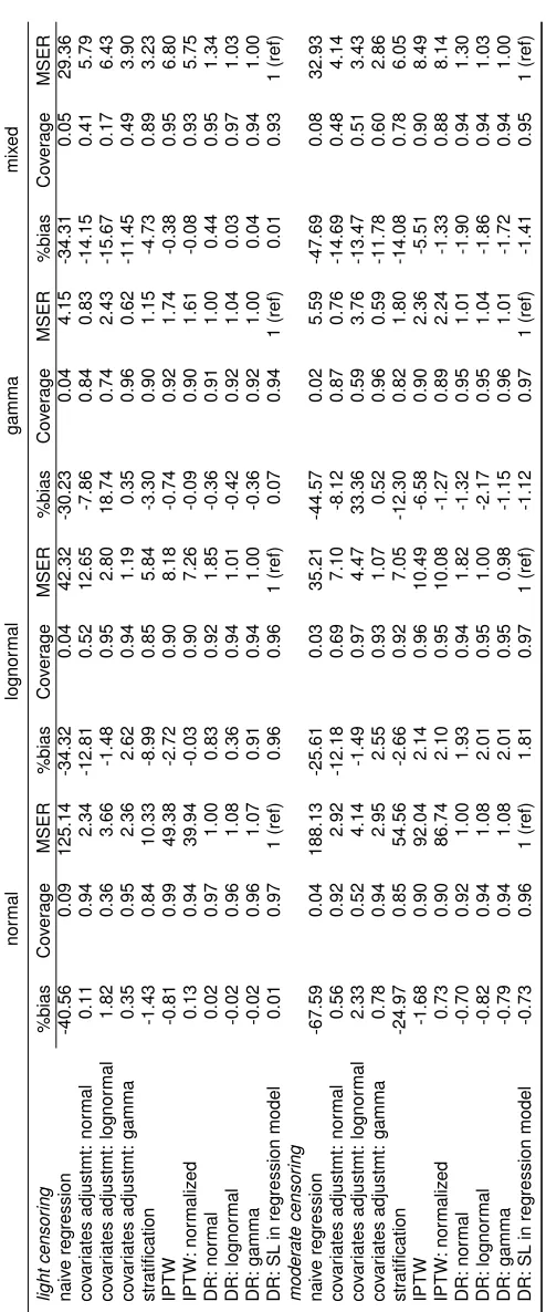
Results of the simulation with various censoring and cost settings and sample size of 1000 appear

in Table 2.1. The naive estimator ignoring censoring and confounders is biased under all settings.

As anticipated, the PS covariate adjustment performs well when the correct model is specified, but

exhibits bias when mis-specified. For example, when cost follows gamma distribution, covariate

adjustment with gamma model yields0.35%bias while the lognormal model had18.74%bias under light censoring. If cost comes from a mixture of normal, lognormal and the gamma distributions,

covariate adjustment methods perform poorly since the true relationship between outcome and PS

is unknown. Of the covariate adjustment models, the gamma model is the most robust, with the

smallest biases for misspecifed cost distributions, a finding consistent with Dodd et al. (2006) and

Basu, Manning, and Mullahy (2004). The PS stratification estimator has large biases and worst

MSE among all PS methods. Note that stratification is most susceptible to under-estimation ofµ.

Since we need to calculate stratum and treatment specificKˆ(u),Kˆ(u)is more likely to be zero for observations with large observation timeT.

IPTW estimators yield bias ranging from -0.38% to -6.58%. The normalized IPTW estimator has

smaller bias than the typical IPTW, consistent with findings from Lunceford and Davidian (2004).

Estimates from DR methods had very small bias, even when the regression model is mis-specified.

Since the PS is correctly modeled, DR estimators should be unbiased due to their doubly robust

property as demonstrated here. Correct regression model specification in DR has very small effect

on bias and coverage since PS model is already correct. Nevertheless, using SL for the regression

model results in small bias and MSE among all DR models. Simulations with a sample size of 5000

(data not shown) produce similar results in terms of bias and coverage, but have smaller MSE. As

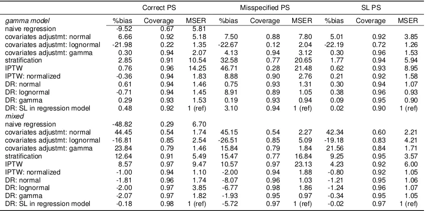
2.6.2. Misspecified PS

Next, we explore the case of PS misspecification when the correct model is unknown. We use the

same simulation procedure as above changing Equation 2.21 to

logit(p) =−2−0.2X1−0.4X2−0.2X3+ 1.4X1X2−1.4X1X3+ 1.2X32 (2.22)

In the simulated data, we estimated PS according to the correct model in Equation 2.22, and also a

misspecified PS model with only main effects ofX1,X2andX3. Finally, we used SL to estimate PS

using all possible combinations of the second order polynomials ofXand the two way interactions

among them. Table 2.2 shows the results for weibull survival time, light censoring, sample size of

1000, gamma and mixed cost models.

Correct PS Misspecified PS SL PS

gamma model %bias Coverage MSER %bias Coverage MSER %bias Coverage MSER

naive regression -9.52 0.67 5.81

covariates adjustmt: normal 6.66 0.92 5.18 7.50 0.88 7.80 5.01 0.92 3.85 covariates adjustmt: lognormal -21.98 0.22 1.35 -22.67 0.12 2.04 -22.19 0.72 1.26 covariates adjustmt: gamma 0.30 0.94 2.07 4.13 0.94 3.12 0.30 0.96 1.53 stratification 2.85 0.91 10.54 32.58 0.77 20.65 1.77 0.94 5.94

IPTW 0.76 0.96 14.25 46.71 0.28 21.48 0.62 0.93 8.95

IPTW: normalized -0.36 0.94 1.83 8.88 0.90 2.76 0.21 0.92 1.58 DR: normal 0.61 0.94 1.46 0.75 0.93 1.31 0.30 0.94 1.07 DR: lognormal -0.71 0.94 1.45 8.91 0.89 1.05 0.38 0.96 0.93 DR: gamma 0.29 0.93 1.53 0.19 0.93 0.94 0.09 0.95 0.90 DR: SL in regression model 0.48 0.92 1 (ref) 3.10 0.94 1 (ref) 0.02 0.90 1 (ref)

mixed

naive regression -48.82 0.29 6.70

covariates adjustmt: normal 44.45 0.54 1.74 45.15 0.54 2.27 42.34 0.60 2.21 covariates adjustmt: lognormal -16.81 0.85 2.54 -26.51 0.85 5.09 -19.18 0.83 4.21 covariates adjustmt: gamma 23.84 0.79 1.46 15.84 0.79 1.84 21.56 0.84 1.71 stratification 12.64 0.91 5.49 15.47 0.77 16.84 9.25 0.95 3.57

IPTW 8.57 0.97 9.47 10.57 0.97 23.13 4.23 0.92 6.00

IPTW: normalized -1.00 0.94 1.10 -2.00 0.94 1.88 -0.80 0.92 1.05 DR: normal -1.81 0.96 1.74 -8.07 0.96 1.03 -1.21 0.95 1.06 DR: lognormal -2.00 0.97 3.85 -6.77 0.98 1.86 -1.24 0.96 1.07 DR: gamma -2.07 0.97 1.82 -1.93 0.95 0.97 -0.34 0.95 1.05 DR: SL in regression model -0.18 0.98 1 (ref) -5.72 0.97 1 (ref) -0.02 0.97 1 (ref)

Table 2.2: %Bias, coverage and relative efficiency for estimated treatment effect on cost under different PS estimation methods

When the PS model is mis-specified, estimates from PS covariate adjustment are biased (4.13%

to 45.15%). Estimates from IPTW methods are also highly biased (-2.00% to 46.71%) when PS

model is mis-specified, in line with Rubin (2004). When the regression models in DR are correctly

established, DR estimators have very small bias. However, when both the regression model and

the PS model are wrong, as anticipated we see some bias (0.75% to 8.91%). Overall, PS

only method that is robust to PS misspecification is DR, provided the regression model is correctly

established.

When SL is used to estimate PS, we see significant improvement of performance across all

estima-tors. In most cases, using SL in PS estimation yields less bias and better coverage than when the

correct PS model is used. Hence, we recommend using SL when the correct PS model is unknown.

When true cost comes from a mixture of normal, lognormal and gamma distributions, SL in DR can

provide the best regression model estimates. In real life settings, it is highly likely that cost comes

from a mixture of different distributions and the correct PS model is unknown. In this case, using

SL with DR and PS estimation provides added flexibility which improves estimates substantially.

2.7. Costs of Bladder Cancer Therapies

Bladder cancer affects more than 70,000 people annually in the United States and accounts for

almost 5% of the total cancer-related costs to Medicare. The guideline recommended treatment for

bladder cancer is radical cystectomy (RC) which involves surgical removal of the bladder. Bladder

preservation therapy (BPT) is a less aggressive, non-surgical alternative that involves radiation and

chemotherapy. Recent studies have shown that BPT may improve quality of life over RC (Efstathiou

et al., 2012). We have applied our method to compare the life-time cost of RC and BPT using a

cohort of patients derived from SEER-Medicare registry.

We included stage II/III bladder cancer patients diagnosed between 1995 and 2005. See Bekelman

et al. (2013) for a detailed description of inclusion/exclusion criterion. 32% of the study cohort

were censored at the end of the study. Payment data were extracted from Carrier Claims file, the

Outpatient file, and the Medicare Provider Analysis and Review Record. We adjusted all costs to

year 2000 dollars using the Medicare Economics Index (Centers for Medicare and Medicaid, 2010).

The final cohort sample size was 1860; 422 had BPT and 1438 had RC. The mean uncensored

costs were $68,800 for BPT patients and $83,040 for RC patients. Total treatment cost were highly

right skewed Figure 2.1 with a maximum observed cost of $511,200. The average observation time

was 3.93 years.

In this study, both treatment assignment and total cost may have been affected by covariates such

Figure 2.1: Density of uncensored total costs in bladder cancer cohort

0

10000

20000

30000

40000

50000

0.86

0.90

0.94

0.98

Willingness to pay ($/yr)

Proportion of iterations with NMB>0

community size. Hence, we estimated PS using a logistic regression model that was adjusted for all

of these potential confounders. We then estimated the difference in total cost between BPT and RC

using the approaches described above including: PS covariates adjustment with normal,

lognor-mal and gamma models, stratification, IPTWs, DR with norlognor-mal, lognorlognor-mal and gamma regression

models and DR using SL in regression model. Naive linear regression ignoring censoring and

non-random treatment assignment was used as a reference. Approximate confidence intervals for the

treatment effect on cost were constructed using non-parametric bootstrapping with BCa correction.

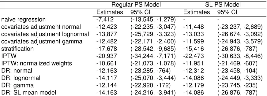
From Table 2.3, BPT was estimated to be $7,412 cheaper than RC using naive regression.

Differ-ence in cost estimated from various propensity score methods ranged from -$10,661 to -$20,937,

differed significantly from the naive regression method. Failure to account for censoring and the

effect of confounders could lead to biased estimates. Furthermore, covariate adjustment,

Regular PS Model SL PS Model

Estimates 95% CI Estimates 95% CI

naive regression -7,412 (-13,545, -1,279) -

-covariates adjustment normal -12,423 (-22,235, -3,047) -11,448 (-23,237, -2,689) covariates adjustment lognormal -13,877 (-25,729, -3,323) -13,033 (-26,674, -3,092) covariates adjustment gamma -12,482 (-22,171, -2,400) -11,599 (-24,943, -3,579)

stratification -17,678 (-28,542, -9,685) -15,416 (-26,876, -787)

IPTW -20,937 (-34,244, -7,171) -22,473 (-30,633, -8,446)

IPTW: normalized weights -10,661 (-21,073, -1,078) -11,951 (-21,469, -607)

DR: normal -12,163 (-23,285, -764) -12,312 (-23,458, -104)

DR: lognormal -14,117 (-25,070, -3,444) -14,086 (-24,449, -3,333)

DR: gamma -12,144 (-22,920, -172) -12,179 (-23,745, -235)

DR: SL mean model -14,163 (-24,216, -3,941) -14,086 (-26,876, -787)

Table 2.3: Estimated mean cost difference for bladder preserving therapy and radical cyccwetomy

we saw large variation in treatment effect estimates from these models. DR models yielded more

consistent treatment effect estimates; BPT was estimated to be -$12,144 to -$14,117 cheaper than

RC. Using SL in regression model in DR gave slight different estimations (-$14,163). SL in

re-gression model in DR is likely to be the closest to the true cost estimate as evidenced from the

simulation study. Lastly, all CIs did not cross zero, indicating that BPT was significantly less costly

than RC.

Next we applied SL in propensity score model to obtain the estimated PS. We specify several

po-tential propensity score models with different covariates functional forms: the basic logistic model

where all covariates were included, also a model including all two way interactions between

co-variates, adding square terms of all covariates and a backwards stepwise selection algorithm with

cut-off p-value of 0.1. SL was used to find the optimal combination of predications from these

can-didate models. We then use this estimated PS to find the differences in cost between BPT and

RC.

From Table 2.3, the SL PS models provided similar estimates from the regular PS models. One

possible explanation is all covariates were categorical, hence there was little variation in PS due to

limited covariate patterns. Interaction and quadratic terms might not have a huge impact on PS

esti-mation for the same reason. SL PS model would be more useful when we have little understanding

of the true PS model. Nevertheless, SL PS showed that the estimates of cost differences were

between -$11,448 and -$22,473, and 95% CIs strongly suggest the differences in cost between

All of the approaches discussed above demonstrate that BPT substantially decreases the total

medical cost compared to the standard treatment RC. However, we observed significant variations

in the ATE estimations and large range in the CIs. From our simulation studies, we believe DR with

SL in both regression model and PS model provides the best estimate. Hence, our findings indicate

that BPT was $14,086 ($787, $26,876) cheaper than RC.

2.8. Discussion

In this study, we explored propensity score based approaches for estimating the treatment effect

on censored costs in an observational study. We extended covariate adjustment, stratification,

weighting and doubly robust methods to handle censored medical cost. We also utilized a machine

learning algorithm, Super Learner, to better estimate PS and the regression models in DR. Our

simulation studies showed that when PS is correctly modeled, stratification and weighting yield

unbiased estimates. Covariate adjustment is sensitive to the choice of outcome model, while DR

is more robust to misspecification. When the correct PS model is unknown, misspecification could

result in biased estimates of the treatment effect even when using DR methods. SL mitigates this

bias by producing optimal regression models and PS estimates. In addition, one may consider

tree-based methods, random forests and neural networks. These methods can be easily incorporated

into SL to obtain optimal PS estimation from both fully parametric and non parametric models.

We note that in this study, we only used total cost data and ignored cost history data which may be

available from claims data. Bang and Tsiatis (2000) have proposed partitioned estimators making

use of cost history data which they showed to be more efficient than the simple weighted approach

we employed. It is unclear what the effect of partitioned estimators would have on PS-based

esti-mation and is worthy of future work.

We have shown that the variance of the IPTW estimator can be obtained analytically. However,

multi-parameter or non-parametric survival models add substantial complexity to analyzing variance

estimates due to the complex interaction between censoring and propensity scores.

As in any observational study, unobserved or hidden bias may be of concern. We suggest that in

addition to a propensity score based analysis of censored cost data, one should conduct a carefully