Menzies Building
Monash University Wellington Road
CLAYTON Vic 3168 AUSTRALIA
Telephone:
(03) 9905 2398, (03) 9905 5112
from overseas:
61 3 9905 5112
Fax numbers:
from overseas:
(03) 9905 2426, (03) 9905 5486
61 3 9905 2426 or
61 3 9905 5486
[email protected]
T
HE
T
HEORETICAL
S
TRUCTURE OF
MONASH-MRF
by
M
atthew
W. P
ETER
M
ark
H
ORRIDGE
G. A. M
EAGHER
F
azana
N
AQVI
and
B.R. P
ARMENTER
Centre of Policy Studies, Monash University
Preliminary Working Paper No. OP-85 April 1996
ISSN 1 031 9034 ISBN 0 7326 0737 X
The Centre of Policy Studies (COPS) is a research centre at Monash University devoted to quantitative analysis of issues relevant to Australian economic policy. The Impact Project is a cooperative venture between the Australian Federal Government and Monash University, La Trobe University, and the Australian National University. COPS and Impact are operating as a single unit at Monash University with the task of constructing a new economy-wide policy model to be known as MONASH. This initiative is supported by the Industry Commission on behalf of the Commonwealth Government, and by several other sponsors. The views expressed herein do not necessarily represent those of any sponsor or government.
C
ENTRE
of
P
OLICY
S
TUDIES
and
the
I
MPACT
i
This paper presents the theoretical specification of the
MONASH-MRF model. MONASH-MONASH-MRF is a multiregional multisectoral model of the
Australian economy. Included is a complete documentation of the model's
equations, variables and coefficients. The documentation is designed to
allow the reader to cross-reference the equation system presented in this
paper in ordinary algebra, with the computer implementation of the model
in the TABLO language presented in CoPS/I
MPACT
Preliminary Working
Paper No. OP-82.
Keywords: multiregional, regional modelling, CGE, regional and Federal
government finances.
ii
ABSTRACT
i
1.
ACKNOWLEDGEMENT AND EXPLANATION
1
2.1
INTRODUCTION
1
2.2
THE CGE CORE
5
2.2.1
Production: demand for inputs to the production process
8
2.2.2
Demands for investment goods
13
2.2.3
Household demands
15
2.2.4
Foreign export demands
17
2.2.5
Government consumption demands
18
2.2.6
Demands for margins
18
2.2.7
Prices
18
2.2.8
Market-clearing equations for commodities
19
2.2.9
Indirect taxes
20
2.2.10
Regional incomes and expenditures
21
2.2.11
Regional wages
23
2.2.12
Other regional factor-market definitions
23
2.2.13
Other miscellaneous regional equations
24
2.2.14
National aggregates
24
2.3
GOVERNMENT FINANCES
24
2.3.1
Disaggregation of value added
27
2.3.2
Gross regional domestic product and its components
29
2.3.3
Miscellaneous equations
30
2.3.4
Summary of financial transactions of the regional and
Federal governments: the SOFT accounts
33
2.3.5
Household disposable income
38
2.4
DYNAMICS FOR FORECASTING
40
2.4.1
Industry capital and investment
42
2.4.2
Accumulation of national foreign debt
47
2.5
REGIONAL POPULATION AND REGIONAL LABOUR
MARKET SETTINGS
50
iii
Table 2.1:
The MMRF Equations
54
Table 2.2:
The MMRF Variables
87
Table 2.3:
The MMRF Coefficients and Parameters
102
Table 2.4:
Dimensions of MMRF
118
LIST OF FIGURES
Figure 2.1:
The CGE core input-output database
6
Figure 2.2:
Production technology for a regional sector in MMRF
9
Figure 2.3:
Structure of investment demand
14
Figure 2.4:
Structure of household demand
16
Figure 2.5:
Government finance block of equations
26
Figure 2.6:
Components of regional value added
28
Figure 2.7:
Income-side components of gross regional product
30
Figure 2.8:
Expenditure-side components of gross regional product
31
Figure 2.9:
Summary of Financial Transaction (SOFT): income side
34
Figure 2.10: Summary of Financial Transaction (SOFT): expenditure side
37
Figure 2.11: Household disposable income
39
Figure 2.12: Comparative-static interpretation of results
41
The Theoretical Structure of
MONASH-MRF
1. Acknowledgement and explanation
This document contains a draft version of chapter 2 from the forthcoming monograph, MONASH-MRF: A Multiregional Multisectoral Model of the Australian Economy. The MONASH-MRF project was initiated in mid 1992 with the sponsorship of the NSW and Victorian State government Treasuries. The authors thank P. B. Dixon, W. J. Harrison and K. R. Pearson for their helpful advice.
2.1. Introduction
MMRF divides the Australia economy into eight regional economies representing the six States and two Territories. There are four types of agent in the model: industries, households, governments and foreigners. In each region, there are thirteen industrial sectors. The sectors each produce a single commodity and create a single type of capital. Capital is sector and region specific. Hence, MMRF recognises 104 industrial sectors, 104 commodities and 104 types of capital. In each region there is a single household and a regional government. There is also a Federal government. Finally, there are foreigners, whose behaviour is summarised by demand curves for regional international exports and supply curves for regional international imports.
In common with the stylised multiregional model described in Chapter 1, in
MMRF, regional demands and supplies of commodities are determined through optimising behaviour of agents in competitive markets. Optimising behaviour also determines demands for labour and capital. National labour supply can be determined in one of two ways. Either by demographic factors or by labour demand. National capital supply can also be determined in two ways. Either it can be specified exogenously or it can respond to rates of return. Labour and capital can cross regional borders in response to labour-market and capital-market conditions.
The specifications of supply and demand behaviour coordinated through market clearing conditions, comprise the CGE core of the model. In addition to the CGE core are blocks of equations describing: (i) regional and Federal
government finances; (ii) accumulation relations between capital and investment, population and population growth, foreign debt and the foreign balance of trade, and; (iii) regional labour market settings.
Computing solutions for MMRF
MMRF is in the Johansen/ORANI class of models1 in that its structural
equations are written in linear (percentage-change) form and results are
1 For an introduction to the Johansen/ORANI approach to CGE modelling, see Dixon,
deviations from an initial solution. Underlying the linear representation of MMRF
is a system of non-linear equations solved using GEMPACK. GEMPACK (see Harrison and Pearson 1994) is a suite of general purpose programs for imple-menting and solving general and partial equilibrium models. A percentage-change version of MMRF is specified in the TABLO syntax which is similar to ordinary algebra.2 GEMPACK solves the system of nonlinear equations arising
from MMRF by converting it to an Initial Value problem and then using one of the standard methods, including Euler and midpoint (see, for example, Press, Flannery, Teukolsky and Vetterling 1986), for solving such problems.
Writing down the equation system of MMRF in a linear (percentage-change) form has advantages from computational and economic standpoints. Linear systems are easy for computers to solve. This allows for the specification of detailed models, consisting of many thousands of equations, without incurring computational constraints. Further, the size of the system can be reduced by using model equations to substitute out those variables which may be of secondary importance for any given experiment. In a linear system, it is easy to rearrange the equations to obtain explicit formulae for those variables, hence the process of substitution is straightforward.
Compared to their levels counterparts, the economic intuition of the percentage-change versions of many of the model's equations is relatively transparent.3 In addition, when interpreting the results of the linear system,
simple share-weighted relationships between variables can be exploited to perform back-of the-envelope calculations designed to reveal the key cause-effect relationships responsible for the results of a particular experiment.
The potential cost of using a linearised representation is the presence of linearisation error in the model's results when the perturbation from the initial solution is large. As mentioned above, GEMPACK overcomes this problem by a multistep solution procedure such a Euler or midpoint. The accuracy of a solution is a positive function of the number of steps applied. Hence, the degree of desired accuracy can be determined by the model user in the choice of the number of steps in the multistep procedure.4
Notational and computational conventions
In this Chapter we present the percentage-change equations of MMRF. Each MMRF equation is linear in the percentage-changes of the model's variables. We
distinguish between the percentage change in a variable and its levels value by
2 The TABLO version of MMRF is presented in the Appendix to Chapter 3.
3 See Horridge, Parmenter and Pearson (1993) for an example based on input demands
given CES production technology.
4 See Harrison and Pearson (1994) for an introduction to the solution methods (including
using lower-case script for percentage change and upper-case script for levels. Our definition of the percentage change in variable X is therefore written as
x = 100
∆X
XIn deriving the percentage-change equations from the nonlinear equations, we use three rules:
the product rule, X = βYZ ⇒ x = y + z, where β is a constant, the power rule, X = βYα⇒ x = αy, where α and β are constants, and the sum rule, X = Y + Z ⇒ Xx = Yy + Zz.
As mentioned above, the MMRF results are reported as percentage deviations in
the model's variables from an initial solution. With reference to the above equations, the percentage changes x, y and z represent deviations from their levels values X, Y and Z. The levels values (X, Y and Z) are solutions to the models underlying levels equations. Using the product-rule equation as an example, values of 100 for X, 10 for Y and 5 for Z represent an initial solution for a value of 2 for β. Now assume that we perturb our initial solution by increasing the values of Y and Z by 3 per cent and 2 per cent respectively, i.e., we set y and z at 3 and 2. The linear representation of the product-rule equation would give a value of x of 5, with the interpretation that the initial value of X has increased by 5 per cent for a 3 per cent increase in Y and a 2 per cent increase in Z. Values of 5 for x, 3 for y and 2 for z in the corresponding percentage change equation means that the levels value of X has been perturbed from 100 to 105, Y from 10 to 10.3 and Z from 5 to 5.1.
(i.e., 100 × 0.15/10.155) and the percentage change in z is 0.9901 per cent (i.e.,
100 × 0.05/5.05), giving a value for x (in our second step) of 2.4679 per cent. Updating our intermediate value of X by 2.4679 per cent, gives a final value of X of 105.045, which is close to the solution of the nonlinear equation of 105.06. We can further improve the accuracy of our solution by implementing more steps and by applying an extrapolation procedure.
In the percentage-change form of the power-rule equation, a constant α appears as a coefficient. In the percentage-change form of the sum-rule equation, the levels values of the variables appear as coefficients. By dividing by X, this last equation can be rewritten so that x is a share-weighted average of y and z. There are two main types of coefficients in the linear equation system of MMRF: (i) price elasticities and (ii) shares of levels values of variables. Two price elasticity coefficients appear in MMRF: elasticities of substitution and own-price elasticities.6 In the MMRF equation system, elasticities of substitution are
identified by the Greek symbol, σ, and own-price elasticities are identified by the prefix ELAST. Equations with share coefficients are typically written in the form of the sum-rule equation above. Coefficients associated with shares are levels values and therefore are written in upper-case script.
The percentage-change equation system of MMRF is given in Table 2.1. The
equations of Table 2.1 are presented in standard algebraic syntax. Each equation has an identifier beginning with the prefix E_. Using the equation identifiers, the reader can cross reference the equations in Table 2.1 with the equations of the annotated TABLO file in the Appendix to Chapter 3. In Table 2.1, below the identifier in brackets, the section in which the equation appears in the annotated
TABLO file is listed. The annotated TABLO file of Chapter 3 is a reproduction of the computer implementation of MMRF. The model's variables are listed in Table 2.2. Descriptions of the model's coefficients appear in Table 2.3, and Table 2.4 describes the sets used in the model.
The remainder of this Chapter is devoted to the exposition of the MMRF
equation system beginning, in section 2.2, with the equations of the CGE core.
5 Note that in our first step we have also updated the values of Y and Z, e.g., after the first
step, our updated value of Y is 10.15 = 10×1.5/100.
6 For example, if, in the power-rule equation, X is quantity demanded and Y is the price of
2.2. The CGE core7
The CGE core is based on ORANI, a single-region model of Australia (Dixon, Parmenter, Sutton and Vincent 1982). Each regional economy in MMRF
looks like an ORANI model. However, unlike the single-region ORANI model, MMRF includes interregional linkages. The transformation of ORANI into the CGE
core of MMRF, in principle, follows the steps by which the stylised single-region
model of Chapter 1 was transformed into the stylised multiregional model. A schematic representation of the CGE core
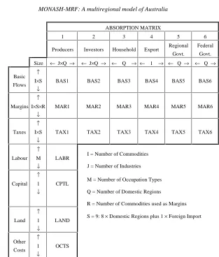
Figure 2.1 is a schematic representation of the CGE core's input-output database. It reveals the basic structure of the CGE core. The columns identify the following agents:
(1) domestic producers divided into J industries in Q regions; (2) investors divided into J industries in Q regions;
(3) a single representative household for each of the Q regions; (4) an aggregate foreign purchaser of exports;
(5) an other demand category corresponding to Q regional governments; and (6) an other demand category corresponding to Federal government demands in
the Q regions.
The rows show the structure of the purchases made by each of the agents identified in the columns. Each of the I commodity types identified in the model can be obtained within the region, form other regions or imported from overseas. The source-specific commodities are used by industries as inputs to current production and capital formation, are consumed by households and governments and are exported. Only domestically produced goods appear in the export column. R of the domestically produced goods are used as margin services (domestic trade and transport & communication) which are required to transfer commodities from their sources to their users. Commodity taxes are payable on the purchases. As well as intermediate inputs, current production requires inputs of three categories of primary factors: labour (divided into M occupations), fixed capital and agricultural land. The other costs category covers various miscellaneous industry expenses. Each cell in the input-output table contains the name of the corresponding matrix of the values (in some base year) of flows of commodities, indirect taxes or primary factors to a group of users. For example, MAR2 is a 5-dimensional array showing the cost of the R margins services on the flows of I goods, both domestically and imported (S), to I investors in Q regions.
Figure 2.1 is suggestive of the theoretical structure required of the CGE
core. The theoretical structure includes: demand equations are required for our
ABSORPTION MATRIX
1 2 3 4 5 6
Producers Investors Household Export Regional Govt.
Federal Govt. Size ← J×Q → ← J×Q → ← Q → ← 1 → ← Q → ← Q → Basic
Flows
↑
I×S
↓
BAS1 BAS2 BAS3 BAS4 BAS5 BAS6
Margins
↑
I×S×R
↓
MAR1 MAR2 MAR3 MAR4 MAR5 MAR6
Taxes
↑
I×S
↓
TAX1 TAX2 TAX3 TAX4 TAX5 TAX6
Labour
↑
M
↓
LABR I = Number of Commodities J = Number of Industries
Capital
↑
1
↓
CPTL M = Number of Occupation Types Q = Number of Domestic Regions
R = Number of Commodities used as Margins
Land
↑
1
↓
LAND S = 9: 8 × Domestic Regions plus 1 × Foreign Import
Other Costs
↑
1
↓
OCTS
Figure 2.1. The CGE core input-output database
six users; equations determining commodity and factor prices; market clearing equations; definitions of commodity tax rates. In common with ORANI, the equations of MMRF's CGE core can be grouped according to the following
classification:
• producer's demands for produced inputs and primary factors;
• demands for inputs to capital creation;
• household demands;
• government demands;
• demands for margins;
• zero pure profits in production and distribution;
• market-clearing conditions for commodities and primary factors; and
• indirect taxes;
• Regional and national macroeconomic variables and price indices. Naming system for variables of the CGE core
In addition to the notational conventions described above in section 2.1, the following conventions are followed (as far as possible) in naming variables of the CGE core. Names consist of a prefix, a main user number and a source dimension. The prefixes are:
a ⇔ technological change/change in preferences; del ⇔ ordinary (rather than percentage) change; f ⇔ shift variable;
nat ⇔ a national aggregate of the corresponding regional variable; p ⇔ prices;
x ⇔ quantity demanded; xi ⇔ price deflator; y ⇔ investment; z ⇔ quantity supplied. The main user numbers are:
1 ⇔ firms, current production; 2 ⇔ firms, capital creation; 3 ⇔ households;
4 ⇔ foreign exports; 5 ⇔ regional government; 6 ⇔ Federal government
The number 0 is also used to denote basic prices and values. The source dimensions are:
a ⇔ all sources, i.e., 8 regional sources and foreign; r ⇔ regional sources only;
t ⇔ two sources, i.e., a domestic composite source and foreign; c ⇔ domestic composite source only;
o ⇔ domestic/foreign composite source only.
The following are examples of the above notational conventions:
p1a ⇔ price of commodities (p), from all nine sources (a) to be used by firms in current production (1);
x2c ⇔ demand for domestic composite (c) commodities (x) to be used by firms for capital creation.
imp ⇔ imports; lab ⇔ labour;
land ⇔ agricultural land;
lux ⇔ linear expenditure system (supernumerary part); marg ⇔ margins;
oct ⇔ other cost tickets;
prim ⇔ all primary factors (land, labour or capital); sub ⇔ linear expenditure system (subsistence part); Sections 2.2.1 to 2.2.14 outline the structure of the CGE core. 2.2.1. Production: demand for inputs to the production process
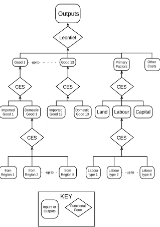
MMRF recognises two broad categories of inputs: intermediate inputs and primary factors. Firms in each regional sector are assumed to choose the mix of inputs which minimises the costs of production for their level of output. They are constrained in their choice of inputs by a three-level nested production technology (Figure 2.2). At the first level, the intermediate-input bundles and the primary-factor bundles are used in fixed proportions to output. These bundles are formed at the second level. Intermediate input bundles are constant-elasticity-of-substitution (CES) combinations of international imported goods and domestic goods. The primary-factor bundle is a CES combination of labour, capital and land. At the third level, inputs of domestic goods are formed as CES
combinations of goods from each of the eight regions, and the input of labour is formed as a CES combination of inputs of labour from eight different
occupational categories. We describe the derivation of the input demand functions working upwards from the bottom of the tree in Figure 2.2. We begin with the intermediate-input branch.
Demands for intermediate inputs
At the bottom of the nest, industry j in region q chooses intermediate input type i from domestic region s (Xi,s,j,q) to minimise the costs
∑
s=1 8
P1Ai,s,j,qX1Ai,s,j,q, i,j=1,...,13 q=1,...,8, (2.1)
of a composite domestic bundle
X1Ci,j,q = CES(X1Ai,1,j,q,...,X1Ai,8,j,q), i,j=1,...,13 q=1,...,8, (2.2)
where the composite domestic bundle (X1Ci,j,q) is exogenous at this level of the
up to
up to from up to Region 8
from Region 2
CES
from Region 1
KEY
Inputs or Outputs
Functional Form
CES CES Leontief
CES CES
Labour type 8 Labour
type 2 Labour
type 1
Capital Labour
Land
Primary Factors
Domestic Good 13 Imported
Good 13 Domestic
Good 1 Imported
Good 1
Good 13 Good 1
Outputs
Other Costs
(1969 1970) specification typically imposed on the use of domestically produced commodities and foreign-imported commodities in national CGE models such as
ORANI.
By solving the above problem, we generate the industries' demand equations for domestically produced intermediate inputs to production.8 The
percentage-change form of these demand equations is given by equations E_x1a1 and E_p1c. The interpretation of equation E_x1a1 is as follows: the commodity demand from each regional source is proportional to demand for the composite X1Ci,j,q and to a price term. The percentage-change form of the price
term is an elasticity of substitution, σ1Ci, multiplied by the percentage change in
a price ratio representing the price from the regional source relative to the cost of the regional composite, i.e., an average price of the commodity across all regional sources. Lowering of a source-specific price, relative to the average, induces substitution in favour of that source. The percentage change in the average price, p1ci,j,q, is given by equation E_p1c. In E_p1c, the coefficient
S1Ai,s,j,q is the cost share in of the ith commodity from the sth regional source in
the jth industry from region q's total cost of the ith commodity from all regional sources. Hence, p1ci,j,q is a cost-weighted Divisia index of individual prices from
the regional sources.
At the next level of the production nest, firms decide on their demands for the domestic-composite commodities and the foreign imported commodities following a pattern similar to the previous nest. Here, the firm chooses a cost-minimising mix of the domestic-composite commodity and the foreign imported commodity
P1Ai,foreign,j,qX1Ai,foreign,j,q + P1Ci,j,qX1Ci,j,q, i,j=1,...,13 q=1,...,8, (2.3)
where the subscript 'foreign' refers to the foreign import, subject to the production function
X1Oi,j,q = CES(X1Ai,foreign,j,q,...,X1Ci,j,q), i,j=1,...,13 q=1,...,8. (2.4)
As with the problem of choosing the domestic-composite, the Armington assumption is imposed on the domestic-composite and the foreign import by the
CES specification in equation 2.4.
The solution to the problem specified by equations 2.3 and 2.4 yields the input demand functions for the domestic-composite and the foreign import represented in their percentage-change form by equations E_x1c, E_x1a2, and E_p1o. The first two equations show, respectively, that the demands for the domestic-composite commodity (X1Ci,j,q) and for the foreign import
8 For details on the solution of input demands given a CES production function, and the
(X1Ai,foreign,j,q) are proportional to demand for the
domestic-composite/foreign-import aggregate (X1Oi,j,q) and to a price term. The X1Oi,j,q are exogenous to the
producer's problem at this level of the nest. Common with the previous nest, the change form of the price term is an elasticity of substitution, σ1Oi, multiplied by
a price ratio representing the change in the price of the domestic-composite (the p1ci,j,q in equation E_x1c) or of the foreign import (the p1ai,foreign,j,q in equation
E_x1a2) relative to price of the domestic-composite/foreign-import aggregate (the p1oi,j,q in equations E_x1c and E_x1a2). The percentage change in the price
of the domestic-composite/foreign-import aggregate, defined in equation E_p1o is again a Divisia index of the individual prices. We now turn our attention to the primary-factor branch of the input-demand tree of Figure 2.2.
Demands for primary factors
At the lowest-level nest in the primary-factor branch of the production tree in Figure 2.2, producers choose a composition of eight occupation-specific labour inputs to minimise the costs of a given composite labour aggregate input. The demand equations for labour of the various occupation types are derived from the following optimisation problem for the jth industry in the qth region.
Choose inputs of occupation-specific labour type m, X1LABOIj,q,m, to
minimise total labour cost
∑
m=1 8
P1LABOIj,q,mX1LABOIj,q,m, j=1,...,13, q=1, ,8, (2.5)
subject to,
EFFLABj,q = CES(X1LABOIj,q,m), j=1,...,13 q,m=1,...,8, (2.4)
regarding as exogenous to the problem the price paid by the jth regional industry for the each occupation-specific labour type (P1LABOIj,q,m) and the regional
industries' demand for the effective labour input (EFFLABj,q).
The solution to this problem, in percentage-change form, is given by equations E_x1laboi and E_p1lab. Equation E_x1laboi indicates that the demand for labour type m is proportional to the demand for the effective composite labour demand and to a price term. The price term consists of an elasticity of substitution, σ1LABj,q, multiplied by the percentage change in a
price ratio representing the wage of occupation m (p1laboij,q,m) relative to the
average wage for labour in industry j of region q (p1labj,q). Changes in the
relative wages of the occupations induce substitution in favour of relatively cheapening occupations. The percentage change in the average wage is given by equation E_p1lab where the coefficients S1LABOIj,q,m are value shares of
occupation m in the total wage bill of industry j in region q. Thus, p1labj,q is a
Divisia index of the p1laboij,q,m. Summing the percentage changes in
each industry gives the percentage change in industry labour demand (labindj,q)
in equation E_labind.
At the next level of the primary-factor branch of the production nest, we determine the composition of demand for primary factors. Their derivation follows the same CES pattern as the previous nests. Here, total primary factor costs
P1LABj,qEFFLABj,q + P1CAPj,qCURCAPj,q + P1LANDj,qNj,q
j = 1,...,13, q = 1,...8, where P1CAPj,q and P1LANDj,q are the unit costs of capital and agricultural
land and CURCAPj,q and Nj,q are industry's demands for capital and agricultural
land, are minimised subject to the production function
X1PRIMj,q = CES
EFFLABj,q
A1LABj,q
, CURCAPj,q
A1CAPj,q
, Nj,q
A1LANDj,q
j = 1,...,13, q = 1,...8, where X1PRIMj,q is the industry's overall demand for primary factors. The
above production function allows us to impose factor-specific technological change via the variables A1LABj,q, A1CAPj,q and A1LANDj,q.
The solution to the problem, in percentage-change form is given by equations E_efflab, E_curcap, E_n and E_xi_fac. From these equations, we see that for a given level of technical change, industries' factor demands are proportional to overall factor demand (X1PRIMj,q) and a relative price term. In
change form, the price term is an elasticity of substitution (σ1FACj,q) multiplied
by the percentage change in a price ratio representing the unit cost of the factor relative to the overall effective cost of primary factor inputs to the jth industry in region q. Changes in the relative prices of the primary factors induce substitution in favour of relatively cheapening factors. The percentage change in the average effective cost (xi_facj,q), given by equation E_xi_fac, is again a cost-weighted
Divisia index of individual prices and technical changes. Demands for primary-factor and commodity composites
We have now arrived at the topmost input-demand nest of Figure 2.2. Commodity composites, the primary-factor composite and 'other costs' are combined using a Leontief production function given by
Zj,q =
1 A1j,q×
MIN
X1Oi,j,q, X1PRIM
j,qA1PRIMj,q
, X1OCTj,q
A1OCTj,q
i,j = 1,...,13, q = 1,...,8. In the above production function, Zj,q is the output of the jth industry in region q,
demands for 'other cost tickets'9 and A1OCT
j,q which are the industry-specific
technological change associated with other cost tickets.
As a consequence of the Leontief specification of the production function, each of the three categories of inputs identified at the top level of the nest are demanded in direct proportion to Zj,q as indicated in equations E_x1o,
E_x1prim and E_x1oct.
2.2.2. Demands for investment goods
Capital creators for each regional sector combine inputs to form units of capital. In choosing these inputs they cost minimise subject to technologies similar to that in Figure 2.2. Figure 2.3 shows the nesting structure for the production of new units of fixed capital. Capital is assumed to be produced with inputs of domestically produced and imported commodities. No primary factors are used directly as inputs to capital formation. The use of primary factors in capital creation is recognised through inputs of the construction commodity (service).
The model's investment equations are derived from the solutions to the investor's three-part cost-minimisation problem. At the bottom level, the total cost of domestic-commodity composites of good i (X2Ci,j,q) is minimised subject
to the CES production function
X2Ci,j,q = CES(X2Ai,1,j,q,...,X2Ai,8,j,q) i,j = 1,...,13 q = 1,...,8,
where the XACi,1,j,q are the demands by the jth industry in the qth region for the
ith commodity from the sth domestic region for use in the creation of capital. Similarly, at the second level of the nest, the total cost of the domestic/foreign-import composite (X2Oi,j,q) is minimised subject the CES
production function
X2Oi,j,q = CES(X2Ai,foreign,j,q,...,X2Ci,j,q), i,j = 1,...,13 q = 1,...,8,
where the X2Ai,foreign,j,q are demands for the foreign imports.
The equations describing the demand for the source-specific inputs (E_x2a1, E_x2a2, E_x2c, E_p2c and E_p2o) are similar to the corresponding equations describing the demand for intermediate inputs to current production (i.e., E_x1a1, E_x1c, E_p1c and E_p2o).
At the top level of the nest, the total cost of commodity composites is minimised subject to the Leontief function
up to
up to from Region 8 from
Region 2
CES
from Region 1
KEY
Inputs or Outputs
Functional Form
Leontief
CES CES
Domestic Good 13 Imported
Good 13 Domestic
Good 1 Imported
Good 1
Good 13 Good 1
Capital Good, Industry j,q
Figure 2.3. Structure of investment demand
Yj,q = MIN
X2Oi,j,q
A2INDi,j,q
i,j = 1,...,13, q = 1,...,8. (2.5)
where the total amount of investment in each industry (Yj,q) is exogenous to the
cost-minimisation problem and the A2INDi,j,q are technological-change
Determination of the number of units of capital to be formed for each regional industry (i.e., determination of Yj,q) depends on the nature of the
experiment being undertaken. For comparative-static experiments, a distinction is drawn between the short run and long run. In short-run experiments (where the year of interest is one or two years after the shock to the economy), capital stocks in regional industries and national aggregate investment are exogenously determined. Aggregate investment is distributed between the regional industries on the basis of relative rates of return.
In long-run comparative-static experiments (where the year of interest is five or more years after the shock), it is assumed that the aggregate capital stock adjusts to preserve an exogenously determined economy-wide rate of return, and that the allocation of capital across regional industries adjusts to satisfy exogenously specified relationships between relative rates of return and relative capital growth. Industries' demands for investment goods is determined by exogenously specified investment/capital ratios.
MMRF can also be used to perform forecasting experiments. Here, regional industry demand for investment is determined by an assumption on the rate of growth of industry capital stock and an accumulation relation linking capital stock and investment between the forecast year and the year immediately following the forecast year.
Details of the determination of investment and capital are provided in section 2.x. below.
2.2.3. Household demands
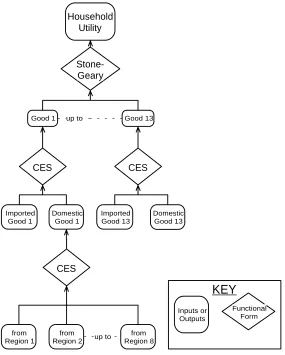
Each regional household determines the optimal composition of its consumption bundle by choosing commodities to maximise a Stone-Geary utility function subject to a household budget constraint. A Keynesian consumption function determines regional household expenditure as a function of household disposable income.
Figure 2.4 reveals that the structure of household demand follows nearly the same nesting pattern as that of investment demand. The only difference is that commodity composites are aggregated by a Stone-Geary, rather than a Leontief function, leading to the linear expenditure system (LES).
The equations for the two lower nests (E_x3a1, E_x3a2, E_x3c, E_p3c and E_p3o) are similar to the corresponding equations for intermediate and investment demands.
up to
up to from Region 8 from
Region 2
CES
from Region 1
KEY
Inputs or Outputs
Functional Form
Stone-Geary
CES CES
Domestic Good 13 Imported
Good 13 Domestic
Good 1 Imported
Good 1
Good 13 Good 1
Household Utility
Figure 2.4. Structure of household demand
demand, which is determined by the Stone-Geary nest of the structure, differ form the CES pattern established in sections 2.2.1 and 2.2.2.10 To analyse the
Stone-Geary utility function, it is helpful to divide total consumption of each commodity composite (X3Oi,q) into two components: a subsistence (or
minimum) part (X3SUBi,q) and a luxury (or supernumerary) part (X3LUXi,q)
10 For details on the derivation of demands in the LES, see Dixon, Bowles and Kendrick
X3Oi,q = X3SUBi,q + X3LUXi,q, i = 1,...,13, q = 1,...,8. (2.6)
A feature of the Stone-Geary function is that only the luxury components effect per-household utility (UTILITY), which has the Cobb-Douglas form
UTILITYq =
1 QHOUSq
∑
i=113
X3LUXi,q A3LUXi,q
q = 1,...,8, (2.7)
where
∑
i=1 13
A3LUXi,q = 1 q = 1,...,8.
Because the Cobb-Douglas form gives rise to exogenous budget shares for spending on luxuries
P3Oi,qX3LUXi,q = A3LUXi,qLUXEXPq i = 1,...,13 q = 1,...,8, (2.8)
A3LUXi,q may be interpreted as the marginal budget share of total spending on
luxuries (LUXEXPq). Rearranging equation (2.8), substituting into equation
(2.6) and linearising gives equation E_x3o, where the subsistence component is proportional to the number of households and to a taste-change variable (a3subi,q), and ALPHA_Ii,q is the share of supernumerary expenditure on
commodity i in total expenditure on commodity i. Equation E_utility is the percentage-change form of the utility function (2.7).
Equations E_a3sub and E_a3lux provide default settings for the taste-change variables (a3subi,q and a3luxi,q), which allow for the average budget
shares to be shocked, via the a3comi,q, in a way that preserves the pattern of
expenditure elasticities.
The equations just described determine the composition of regional household demands, but do not determine total regional consumption. As mentioned, total household consumption is determined by regional household disposable income. The determination of regional household disposable income and regional total household consumption is described in section 2.xx.
2.2.4. Foreign export demands
To model export demands, commodities in MMRF are divided into two groups: the traditional exports, agriculture and mining, which comprise the bulk of exports; and the remaining, non-traditional exports. Exports account for relatively large shares in total sales of agriculture and mining, but for relatively small shares in total sales for non-traditional-export commodities.
The traditional-export commodities (X4Ri,s, i∈agricult,mining) are
X4Ri,s = FEQi
P4Ri,s
FEPiNATFEP
EXP_ELASTi
i = 1, 2, s = 1,...,13, (2.9)
where EXP_ELASTi is the (constant) own-price elasticity of foreign-export
demand. As EXP_ELASTi is negative, equation (2.9) says that traditional
exports are a negative function of their prices on world markets (P4Ri,s). The
variables FEQi and FEPi allow for horizontal (quantity) and vertical (price)
shifts in the demand schedules. The variable NATFEP allows for an economy-wide vertical shift in the demand schedules. The percentage-change form of (2.9) is given by E_x4r.
In MMRF the commodity composition of aggregate non-traditional exports is exogenised by treating non-traditional exports as a Leontief aggregate (equation E_nt_x4r). Total demand is related to the average price via a constant-elasticity demand curve, similar to those for traditional exports (see equations E_aggnt_x4r and E_aggnt_p4r).
2.2.5. Government consumption demands
Equations E_x5a and E_x6a determine State government and Federal government demands (respectively) for commodities for current consumption. State government consumption can be modelled to preserve a constant ratio with State private consumption expenditure by exogenising the 'f5' variables in equation E_x5a. Likewise, Federal government consumption expenditure can be set to preserve a constant ratio with national private consumption expenditure by exogenising the 'f6' variables in equation E_x6a.
2.2.6. Demands for margins
Equations E_x1marg, E_x2marg, E_x3marg, E_x4marg, E_x5marg and E_x6marg give the demands, of our six users, for margins. Two margin commodities are recognised in MMRF: transport & communication and finance. These commodities, in addition to being consumed directly by the users (e.g., consumption of transport when taking holidays or commuting to work), are also consumed to facilitate trade (e.g., the use of transport to ship commodities from point of production to point of consumption). The latter type of demand for transport & communication and finance are the so-called demands for margins. The margin demand equations in MMRF indicate that the demands for margins are proportional to with the commodity flows with which the margins are associated.
2.2.7. Prices
As is typical of ORANI-style models, the price system underlying MMRF
Also in the tradition of ORANI is presence of two types of price equations: (i) zero pure profits in current production, capital creation and importing and (ii) zero pure profits in the distribution of commodities to users. Zero pure profits in current production, capital creation and importing is imposed by setting unit prices received by producers of commodities (i.e., the commodities’ basic values) equal to unit costs. Zero pure profits in the distribution of commodities is imposed by setting the prices paid by users equal to the commodities’ basic value plus commodity taxes and the cost of margins. Zero pure profits in production, capital creation and importing
Equations E_p0a and E_a impose the zero pure profits condition in current production. Given the constant returns to scale which characterise the model’s production technology, equation E_p0a defines the percentage change in the price received per unit of output by industry j of region q (p0a j,q) as a
cost-weighted average of the percentage changes in effective input prices. The percentage changes in the effective input prices represent (i) the percentage change in the cost per unit of input and (ii) the percentage change in the use of the input per unit of output (i.e., the percentage change in the technology variable). These cost-share-weighted averages define percentage changes in average costs. Setting output prices equal to average costs imposes the competitive zero pure profits condition.
Equation E_pi imposes zero pure profits in capital creation. E_pi determines the percentage change in the price of new units of capital (pi j,q) as
the percentage change in the effective average cost of producing the unit. Zero pure profits in imports of foreign-produced commodities is imposed by Equation E_p0ab. The price received by the importer for the ith commodity (P0Ai,foreign) is given as product of the foreign price of the import
(PMi), the exchange rate (NATPHI) and one plus the rate of tariff (the so-called
power of the tariff: POWTAXMi)11.
Zero pure profits in distribution
The remaining zero-pure-profits equations relate the price paid by purchasers to the producer's price, the cost of margins and commodity taxes. Six users are recognised in MMRF and zero pure profits in the distribution of commodities to the users is imposed by the equations E_p1a, E_p2a, E_p3a, E_p4r, E_p5a and E_p6a.
2.2.8. Market-clearing equations for commodities
Equations E_mkt_clear_margins, E_mkt_clear_nonmarg and E_x0impa impose the condition that demand equals supply for domestically-produced margin and nonmargin commodities and imported commodities respectively. The
11 If the tariff rate is 20 percent, the power of tariff is 1.20. If the tariff rate is increased
output of regional industries producing margin commodities, must equal the direct demands by the model's six users and their demands for the commodity as a margin. Note that the specification of equation E_mkt_clear_margins imposes the assumption that margins are produced in the destination region, with the exception that margins on exports and commodities sold to the Federal government are produced in the source region.
The outputs of the nonmargin regional industries are equal to the direct demands of the model's six users. Import supplies are equal to the demands of the users excluding foreigners, i.e., all exports involve some domestic value added.
2.2.9. Indirect taxes
Equations E_deltax1 to E_deltax6 contain the default rules for setting sales-tax rates for producers (E_deltax1), investors (E_deltax2), households (E_deltax3), exports (E_deltax4), and government (E_deltax5 and E_deltax6). Sales taxes are treated as ad valorem on the price received by the producer, with the sales-tax variables (deltax(i), i=1,...,6) being the ordinary change in the percentage tax rate, i.e., the percentage-point change in the tax rate. Thus a value of deltax1 of 20 means the percentage tax rate on commodities used as inputs to current production increased from, say, 20 percent to 40 percent, or from, say, 24 to 44 percent.
For each user, the sales-tax equations allow for variations in tax rates across commodities, their sources and their destinations.
Equations E_taxrev1 to E_taxrev6 compute the percentage changes in regional aggregate revenue raised from indirect taxes. The bases for the regional sales taxes are the regional basic values of the corresponding commodity flows. Hence, for any component of sales tax, we can express revenue (TAXREV), in levels, as the product of the base (BAS) and the tax rate (T), i.e.,
TAXREV = BAS×T. Hence,
∆TAXREV = T∆BAS + BAS∆T (2.10)
The basic value of the commodity can be written as the product the producer's price (P0) and the output (XA)
BAS = P0×XA. (2.11)
TAXREV×taxrev = TAX×(p0 + xa) + BAS×deltax where
taxrev = 100
∆TAXREV
TAXREV ,TAX = BAS×T p0 = 100
∆P0P0
, xa = 100
∆XA
XA . anddeltax = 100×∆T
2.2.10. Regional incomes and expenditures
In this section, we outline the derivation of the income and expenditure components of regional gross product. We begin with the nominal income components.
Income-side aggregates of regional gross product
The income-side components of regional gross product include regional totals of factor payments, other costs and the total yield from commodity taxes. Nominal regional factor income payments are given in equations E_caprev, E_labrev and E_lndrev for payments to capital, labour and agricultural land, respectively. The regional nominal payments to other costs are given in equation E_octrev.
The derivation of the factor income and other cost regional aggregates are straightforward. Equation E_caprev, for example is derived as follows. The total value of payments to capital in region q (AGGCAPq) is the sum of the
payments of the j industries in region q (CAPITALj,q), where the industry
payments are a product of the unit rental value of capital (P1CAPj,q) and the
number of units of capital employed (CURCAPj,q)
AGGCAPq =
∑
j=1 13Equation (2.12) can be written in percentage changes as
caprevq= (1.0/AGGCAPq)
∑
j=1 13CAPITALj,q(p1capj,q + curcapj,q),
q = 1,...,8,
giving equation E_caprev, where the variable caprevq is the percentage change
in rentals to capital in region q and has the definition,
caprevq = 100
∆AGGCAPq
AGGCAPq q = 1,...8.
The regional tax-revenue aggregates are given by equations E_taxind, E_taxrev6 and E_taxrevm. E_taxrev6 has been discussed in section 2.2.9. E_taxind determines the variable taxindq, which is the weighted average of the
percentage change in the commodity-tax revenue raised from the purchases of producers, investors, households, foreign exports and the regional government. Equation E_taxrevm determines tariff revenue on imports absorbed in region q (taxremq). Equation E_taxrevm is similar in form to equations E_taxrev1 to
E_taxrev6 discussed in section 2.2.9. However, the tax-rate term in equation E_taxrevm, powtaxmq, refers to the percentage change in the power of the tariff
(see footnote 2) rather than the percentage-point change in the tax rate (as is the tax-rate term in the commodity-tax equations of section 2.2.9).
Expenditure-side aggregates of regional gross product
For each region, MMRF contains equations determining aggregate expenditure by households, investors, regional government, the Federal government and the interregional and foreign trade balances. For each expenditure component (with the exception of the interregional trade flows), we define a quantity index and a price index and a nominal value of the aggregate. For interregional exports and imports, we define an aggregate price index and quantity index only.
As with the income-side components, each expenditure-side component is a definition. As with all definitions within the model, the defined variable and its associated equation could be deleted without affecting the rest of the model. The exception is regional household consumption expenditure (see equations E_c_a, E_cr and E_xi3). It may seem that the variable cq is determined by the
equation E_c_a. This is not the case. Nominal household consumption is determined either by a consumption function (see equation E_c_b in section xxx) or, say, by a constraint on the regional trade balance. Equation E_c_a therefore plays the role of a budget constraint on household expenditure.
exports, interregional imports, international exports and international imports. The equations defining quantities are E_ir, E_othreal5, E_othreal6, E_int_exp, E_int_imp, E_expvol and E_impvol. The equations describing price indices are E_xi2, E_xi5, E_xi6, E_psexp, E_psimp, E_xi4 and E_xim. The definitions of nominal values are given by equations E_in, E_othnom5, E_othnom6, E_export and E_imp (remembering that the model does not include explicit equations or variables defining aggregate nominal interregional trade flows).
The derivation of the quantity and price aggregates for the interregional trade flows involves an intermediate step represented by equations E_trd and E_psflo. These equations determine inter- and intra- regional nominal trade flows in basic values.12 To determine the interregional trade flows, say for
interregional exports in E_int_exp, the intraregional trade flow (the second term on the RHS of E_int_exp) is deducted from the total of inter- and intra- regional trade flows (the first term on the RHS of E_int_exp).
2.2.11. Regional wages
The equations in this section have been designed to provide flexibility in the setting of regional wages. Equation E_p1laboi separates the percentage change in the wage paid by industry (p1laboij.q,m) into the percentage change in
the wage received by the worker (pwageij.q) and the percentage change in the
power of the payroll tax (arpij.q). Equation E_pwagei allows for the indexing of
the workers' wages to the national consumer price index (natxi3, see section xxx). The 'fwage' variables in E_pwagei allow for deviations in the growth of wages relative to the growth of the national consumer price index.
Equation E_wage_diff allows flexibility in setting movements in regional wage differentials. The percentage change in the wage differential in region q (wag_diffq) is defined as the difference the aggregate regional real
wage received by workers (pwageq - natxi3) and the aggregate real wage
received by workers across all regions (natrealwage). Equation E_pwage defines the percentage change in the aggregate regional nominal wage (pwageq)
as the average (weighted across industries) of the pwageij,q and equation
E_natrealw defines the percentage change in the variable natrealwage. 2.2.12. Other regional factor-market definitions
The equations in this section define aggregate regional quantities and prices in the labour and capital markets.
Equations E_l, E_kt and E_z_tot define aggregate regional employment, capital use and value added respectively. E_lambda defines regional employment of each of the eight occupational skill groups.
12 The determination in basic values reflects the convention in MMRF that all margins and
The remaining equations of this section define aggregate regional prices of labour and capital.
2.2.13. Other miscellaneous regional equations
Equation E_p1oct allows for the indexation of the unit price of other costs to be indexed to the national consumer price index. The variable f1octj.q
can be interpreted as the percentage change in the real price of other costs to industry j in region q.
Equation E_cr_shr allows for the indexing of regional real household consumption with national real household consumption in the case where the percentage change in the regional-to-national consumption variable, cr_shrq is
exogenous and set to zero. Otherwise, cr_shrq is endogenous and regional
consumption is determined elsewhere in the model (say, by the regional consumption function).
Equation E_ximp0 defines the regional duty-paid imports price index. Equation E_totdom and E_totfor define, for each region, the interregional and international terms of trade respectively.
2.2.14. National aggregates
The final set of equations in the CGE core of MMRF define economy-wide variables as aggregates of regional variables. As MMRF is a bottoms-up regional model, all behavioural relationships are specified at the regional level. Hence, national variables are simply add-ups of their regional counterparts.
2.3. Government finances
In this block of equations, we determine the budget deficit of regional and federal governments, aggregate regional household consumption and Gross State Products (GSP). To compute the government deficits, we prepare a summary of financial transactions (SOFT) which contain government income from various sources and expenditure on different accounts. To determine each region's aggregate household consumption, we compute regional household disposable income and define a regional consumption function. The value added in each region is determined within the CGE core of the model. Within the government finance block, are equations which split the regions' value added between private and public income. In this disaggregation process, the GSPs are also computed from the income and expenditure sides. The government finance equations are presented in five groups:
(i) value added disaggregation; (ii) gross regional product; (iii) miscellaneous equations.
Figure 2.5 illustrates the interlinkages between the five government finance equation blocks and their links with the CGE core and regional population and labour market equation block of MMRF. The activity variables and commodity taxes are determined in the CGE core.
From Figure 2.5, we see that all the equation blocks of government finances have backward links to the CGE core. The disaggregation-of-value-added block takes expenditures by firms on factors of production from the CGE
core and disaggregates them into gross returns to factors and production taxes. Regional value added is used in the determination of the income side of gross regional product, hence the link from the value-added block to the gross-regional-product block in Figure 2.5. Production tax revenue also appears as a source of government income in the SOFT accounts block, which explains the link between value-added and SOFT in Figure 2.5. Factor incomes help explain household disposable income and this is recognised by the link between the value-added block and the household-disposable-income block in Figure 2.5.
The miscellaneous block in Figure 2.5 contains intermediary equations between the gross-regional-product block and the SOFT accounts, and between
the household-disposable-income block and the CGE core. There are two types of
equations in the miscellaneous block: (i) aggregating equations that form national macroeconomic aggregates of the expenditure and income sides of GDP by summing the corresponding regional macroeconomic variables determined in the gross-regional-product block and; (ii) mapping equations that rename variables computed in the gross-regional-product block and the CGE core for use in the SOFT accounts.
The SOFT accounts compute the regional and Federal governments' budgets. On the income side are government tax revenues, grants from the Federal government to the regional governments, interest payments and other miscellaneous revenues. Direct taxes and commodity taxes come from the gross-regional-product block via the miscellaneous block as described above. Production taxes come from the value-added block. On the expenditure side of the government budgets are purchases of goods and services, transfer payments, interest payments on debt, and for the Federal government, payments of grants to the regional governments. The purchases of goods and services come from the
Value Added
Gross Regional Product
Miscellaneous Equations
SOFT Accounts
Household Disposable Income CGE
Core & Labour MarketRegional Pop.
KEY
Government finance block of equations.
The five equation groupings within the government finance block.
Other equation blocks that link with government finances.
Direction of link between equation groupings, and other equation blocks.
Figure 2.5. Government finance block of equations
Finally, we come to the household-disposable-income block. Within this block, household disposable income is determined as the difference between the sum of factor incomes and transfer payments, and income taxes. Figure 2.5 shows that factor incomes come from the value-added block and that unemployment benefits are determined using information from the regional population and labour market block. Household disposable income feeds back to the miscellaneous block, which contains an equation specifying the level of regional household consumption as a function of regional household disposable income. The value of regional household consumption, in turn, feeds back to the
CGE core. Also, the value of transfer payments, determined in the household-disposable-income block, feedback to the SOFT accounts.
A notation for the government finance block
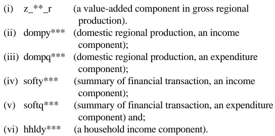
We have given specific notation to variables of each of the blocks which form the government finance set of equations. The following are the major array names for variables and coefficients:
(i) z_**_r (a value-added component in gross regional production).
(ii) dompy*** (domestic regional production, an income component);
(iii) dompq*** (domestic regional production, an expenditure component);
(iv) softy*** (summary of financial transaction, an income component);
(v) softq*** (summary of financial transaction, an expenditure component) and;
(vi) hhldy*** (a household income component).
In each array name '***' represents three or two digits component numbers. In the following sections we discuss the various blocks which constitute the government finance equations of MMRF beginning with the disaggregation of value added.
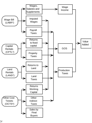
2.3.1. Disaggregation of value added
Figure 2.6 shows that the essential purpose of the disaggregation-of-value-added block is to disaggregate the four elements of value added determined in CGE core (i.e., the wage bill, the rental cost of capital and land, and other costs) into ten components in order to separate production taxes from payments to factors. In addition, the block prepares national values as aggregates of regional values. We now turn to the details of the value-added equation block as presented in section 2.3 of Table 2.1.
In equations E_z01_r and E_z02_r, we assume that the wages, salaries and supplements and the imputed wage bill vary in direction proportion to the pre-tax wage bill, which is determined in the CGE core. Equation E_z03_r shows that payroll taxes are determined by the pre-tax wage bill and the payroll tax rate. Equations E_z04_r and E_z05_r show that the return to fixed capital and property taxes are assumed to vary in proportion to the rental cost of capital, which is determined in the CGE core. Returns to agricultural land and land taxes
are determined by equations E_z06_r and E_z07_r respectively and vary in proportion to the total rental cost of land. Returns to working capital, other indirect taxes and sales by final buyers are all assumed to vary in proportion to other costs. The relevant equations are E_z08_r, E_z09_r and E_z010_r respectively.
Wages, Salaries and Supplements
Imputed Wages
Payroll Taxes
Returns to fixed capital Wage Bill
(LABR*)
Returns to Land
Land Taxes
Returns Working Capital
Other Indirect
Taxes
Sales by Final Buyers Property Taxes Capital
Rentals (CPTL*)
Land Rentals (LAND*)
Other Cost Tickets (OCTS*)
Wage Income
GOS
Production Taxes
Value Added
KEY
* The name in parenthesis indicates the corresponding array name in Figure 2.1. Elements from the CGE Core.
Elements in the disaggregation-of-value-added block.
Equation E_zg_r defines regional gross operating surplus (GOS) as the sum of imputed wages and returns to fixed capital, working capital and agricultural land. Equation E_zt_r calculates total regional production tax revenues.
Equation E_rpr sets the payroll tax rates by industry and region which are determined by the payroll tax rate for all industries in a region and a shift in the industry and region specific payroll tax rate. A change in the payroll tax rate drives a wedge between the wage rate received by the workers and the cost to the producer of employing labour. The change in the cost of employing labour for a given change in the payroll tax rate depends on the share of the payroll taxes in total wages. Equation E_rpri adjusts the payroll tax rate to compute the wedge between the wage rate and labour employment costs. The wedge is used to define the after-tax wage rate in the CGE core.
The last equation in the value-added block, E_xisfb2, defines a regional price index for sales by final buyers.
2.3.2. Gross regional domestic product and its components
This block of equations defines the regional gross products from the income and expenditure sides using variables from the CGE core and the value-added block.
Figure 2.7 reveals that gross regional product at market prices from the income side is sum of wage income, non-wage income and indirect tax revenues.
In section 2.3 of Table 2.1, equations E_dompy100, E_dompy200 and E_dompy330 show, respectively, that wage income, non-wage income and production taxes are mapped from the value-added block. In addition to production taxes, there are two other categories of indirect tax: tariffs and other commodity taxes less subsidies. Equations E_dompy330 and E_dompy320 show that these taxes are mapped from the CGE core. Total indirect taxes are defined by E_dompy300 as the sum of the three categories of indirect taxes.
Summing wage and non-wage income, and indirect taxes gives gross regional product from the income side (equation E_dompy000).
Wage Income
Value Added
Non Wage Income
Production Taxes
Tariffs
Other Commodity Taxes Less Subsidies
Indirect Taxes
Gross Regional
Product
CGE Core
Figure 2.7. Income-side components of gross regional product
Figure 2.8 shows that gross regional product from the expenditure side is defined as the sum of domestic absorption and the interregional and international trade balances. This definition is reflected in equation E_dompq000. Domestic absorption is defined in equation E_dompq100 as the sum of private and public consumption and investment expenditures. Equations E_dompq110 to E_dompq150 reveal that the components of domestic absorption are mapped from the CGE core. Within the components of domestic absorption, the assumption is made, in equations E_dompq120 and E_dompq150, that the shares of private and government investment in total investment are fixed. Equations E_dompq210 and E_dompq220 show that regional exports and imports are also taken from the CGE core. The difference between regional exports and imports forms the regional trade balance and is calculated in equation E_dompq200. Similarly the international trade variables for each region are taken from the CGE core (E_dompq310 and E_dompq320 for international exports and imports respectively) and are used to define the international trade balance for each region in equation E_dompq300.
2.3.3. Miscellaneous equations
Private Consumption
Private Investment
Regional Government Consumption
Federal Government Consumption
Interregional Exports
Interregional Imports
International Exports
International Imports Government
Investment CGE
Core
Domestic Absorption
Interregional Trade Balance
Gross Regional
Product
International Trade Balance
Figure 2.8 Expenditure-side components of gross regional product
then summed, in equation E_yn, to form national nominal GDP. In equation E_xiy_r, a gross-regional-product price deflator from the expenditure side, is formed using price indices taken from the CGE core. The resulting price deflator is used to define real gross regional product in equation E_yr_r.
Taking a weighted average of the gross regional product price deflators gives the price deflator for national GDP in equation E_xiy. This deflator is used to define real national GDP in equation E_yr.
ratio. Note that E_bstar defines a percentage-point change in a ratio, rather than a percentage change. The underlying levels equation of E_bstar is
BSTAR =
∑
q=1 8
DOMPQ300q
YN ,
where the upper-case represents the levels values of the corresponding percentage-point change and percentage change variables. Taking the first difference of BSTAR and multiplying by 100 gives the percentage-point change in BSTAR (i.e., the variable bstar on the LHS of E_bstar)
100×∆BSTAR = bstar =
∑
q=1 8
DOMPQ300qdompq300q
YN -
NATB YN yn, where
NATB =
∑
q=1 8
DOMPQ300q.
Aggregate national income taxes are calculated in equation E_ty. They are the sum of regional PAYE taxes and regional taxes on non-wage income. Pre-tax national wage income is calculated in equation E_yl by summing pre-Pre-tax regional wage incomes. Equation E_wn defines the nominal pre-tax national wage rate as the ratio of the pre-tax wage income to national employment. The nominal post-tax national wage income is calculated in equation E_ylstar by summing the nominal post-tax regional wage incomes. The nominal post-tax national wage rate is defined in equation E_wnstar as the ratio of the nominal post-tax wage income to national employment. The real post-tax national wage rate is defined in E_wrstar by deflating the nominal post-tax national wage rate by the national CPI.
Equations E_g_rA and E_g_rB define the regional government and Federal government consumption expenditures respectively. The vector variable determined in these equations, g_r, drives government consumption expenditures in the SOFT accounts (see section 2.3.4 below).
residual in equation E_ig, as the difference between total aggregate total investment and aggregate private investment. Equation E_ig_reg imposes the assumption that investment expenditure of regional governments moves in proportion to total regional investment. Equation E_ig_r_fed determines investment expenditure of the Federal government as the difference between total public investment and the sum of regional governments' investment.
The miscellaneous equation block is completed with equation E_c_b defining the regional household consumption function and equation E_rl relating the PAYE tax rate to the tax rate on non-wage income.
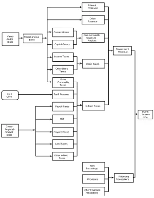
2.3.4. Summary Of Financial Transactions of the regional and Federal governments: the SOFT accounts.
In this block of equations, we prepare a statement of financial transactions containing various sources of government income and expenditure. A separate statement is prepared for each regional government and the Federal government. Our accounting system is based on the State Finance Statistics (cat. no. 5512.0) of the Australian Bureau of Statistics (ABS).
The SOFT accounts contain equations explaining movements in the income and expenditure sides of the governments' budgets. Our exposition of this equation block starts with the income side of the accounts. Figure 2.9 depicts the income side of the SOFT accounts. There are two major categories of
government income: (i) revenues and (ii) financing transactions. Government revenues are further divided into direct and indirect tax revenues, interest payments, Commonwealth grants (for regional governments) and other revenues. The categories of direct taxes are income taxes (for the Federal government), and other direct taxes. Indirect taxes consist of tariffs (for the Federal government), other commodity taxes and production taxes. Commonwealth grants are divided into grants to finance consumption expenditure and grants used to finance capital expenditure. Financing transactions capture the change in the governments' net liabilities and represent the difference between government revenue and government expenditure. If government expenditure exceeds/is less than government revenue (i.e., the government budget is in deficit/surplus), then financing transactions increase/decrease as either the governments' net borrowings increase and/or other financing transactions increase. Variations in the latter item principally consist of changes in cash and bank balances.13 We
now turn our attention to the specification of movements in the income-side
13 The reader will note that financing transactions includes a third item, increase in
Value-Added Block
Miscellaneous Block
Current Grants Capital Grants Income Taxes Other Direct Taxes
Other Commodity
Taxes Tariff Revenue
Payroll Taxes FBT PropertyTaxes
Land Taxes Other Indirect
Taxes
Interest Received
Other Revenue Commonwealth
Grants to Regions Direct Taxes Indirect Taxes
New Borrowings
Provisions Other Financing
Transactions
Government Revenue
SOFT: Income side Financing
Transactions
Gross- Regional-Product
Block CGE Core