AMPLITUDE ONLY PATTERN SYNTHESIS OF ARRAYS USING GENETIC ALGORITHMS

(1)

AMPLITUDE ONLY PATTERN

SYNTHESIS OF ARRAYS USING

GENETIC ALGORITHMS

V. RAJYA LAKSHMI

Department of Electronics and Communication Engineering,

Anil Neerukonda Institute of Technology and Sciences, Visakhapatnam, India

G. S. N RAJU

Department of Electronics and Communications Engineering, AU College of Engineering (A), Andhra University, Visakhapatnam, India

Abstract:

Array pattern synthesis is one of the most important problems in communication and radar applications. The synthesis is usually carried out by controlling amplitude and phase levels (or) element spacing functions of the array. Although, uniform linear arrays cost effective in terms of sources it is not preferred due to high presence of high first side lobe levels i.e. – 13.5dB. For point to the point communications, and high angular resolutions radars, it is essential to generate low side lobe narrow beams. In view of these facts, a linear array is considered in the present work and it is optimally designed using genetic algorithm. The desired amplitude levels are evaluated using the algorithm. The computed amplitude distribution, the realized radiation patterns over specified scan angles are presented.

Key words: Radiation pattern; Side lobe level; null to null beam width; Genetic algorithm.

1. Introduction

In many communication applications, it is required to design a highly directional antenna. Array antennas have high gain and directivity compared to an individual radiating element [1].Antenna array is formed by assembling of radiating elements in an electrical or geometrical configuration. Total field of the antenna array is found by vector addition of the fields radiated by each individual element [2].In an array of identical elements, five controls that can be used to shape the overall pattern of the antenna are geometrical configuration of the overall array, relative displacement between elements, excitation amplitude of individual elements, excitation phase of individual elements, and relative pattern of the individual elements. A linear array has all its elements placed along a straight line with a uniform relative spacing between elements [3].

The first optimum antenna array distribution is the binomial distribution proposed by stone. As is well known, the amplitude weights of the elements in the array correspond to the binomial coefficients and resulting array has no side lobes. Dolph mapped the chebyschev polynomial onto the array factor polynomial to get all the side lobes at an equal level. The resulting array factor polynomial coefficients represent the Dolph -chebyschev amplitude distribution [4]. This amplitude taper is optimum in that specifying the maximum side lobe level results in the smallest beam width or specifying the beam width results in the lowest possible maximum side lobe level. Taylor developed a method to optimize the side lobe levels and beam width of a line source [5]. Elliot extended Taylor’s work to new horizons, including Taylor based tapers with asymmetric side lobe levels, arbitrarily side lobe level designs [6].

(2)

algorithms because they are powerful in solving nonlinear optimization problems. Genetic algorithms have shown great potential in the solution of complex problems related to the design of antennas [7-9].

Low sidelobe antenna arrays are becoming an increasingly important component of high performance electronic systems, particularly those operating in heavy clutter and jamming environments[10].Therefore, the goal in this amplitude only antenna array synthesis is to determine the excitation levels of the array that produces the radiation pattern which suppress the relative sidelobe level with respect to main beam without disturbing the null to null beamwidth for a linear array of isotropic elements. Real genetic algorithm (RGA) is used to get the desired pattern of the array.

2. Genetic Algorithm

Genetic algorithms are global search algorithms based on the mechanics of natural selection and natural genetics. A genetic algorithm is a search technique used in computing to find exact or approximate solutions to optimization and search problems. The central theme of research on genetic algorithm has been robustness, the balance between efficiency and efficacy necessary for survival in many different environments

The difference between genetic algorithm and classical search methods [11] are listed below. GA (1) Optimizes with continuous or discrete parameters

(2) Doesn’t require derivative information

(3) Simultaneously searches from wide sampling of cost surface. (4) Works with large no of variables

(5) Well suited for parallel computers, optimizes variables with extremely complex cost surfaces. (6) May encode parameters and optimization is done with numerically generated data, experimental or

analytical data.

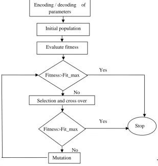
Genes are the basic building blocks of genetic algorithm. A gene is a binary encoding of a parameter .A chromosome is an array of genes. Each chromosome has an associated cost function assigning a relative merit to that chromosome. The genetic algorithm uses the selection, recombination and mutation operators on the population of individuals to perform the search. The population is randomly created at the start of the search. The fitness is used to select individuals from the current generations to advance into the next generation. These individuals are recombined and possibly mutated to form the next generation. This process is continued until there is no change in the best individual in the population. The flow chart of genetic algorithm is presented in Fig. 1. for the sake of completeness.

Selection begins by determining the relative fitness of each individual. This selection process continues until a new population is formed. The algorithm begins with a large list of random chromosomes. Cost functions are evaluated for each chromosome. The chromosomes are ranked from the fit to the last fit according to their respective cost functions. Unacceptable chromosomes are discarded leaving a superior species subset of the original list. Genes that survive become parents, by swapping some of their genetic material to produce two new offspring.

The parents reproduce enough to offset the discarded chromosomes. Thus the total number of chromosomes remains constant after each iteration. Mutations cause small random changes in a chromosome. Cost functions are evaluated for the offspring and the mutated chromosome and the process is repeated .The algorithm stops after a set number of iterations or when a acceptable solution is obtained.

2.1.GA operators

Once a pair of individuals has been selected as parents, a pair of children is created by recombining and mutating the chromosomes of the parents utilizing the basic genetic algorithm operators crossover and mutation. Cross over and mutations are applied with probability pcross and pmutation respectively.

2.2.Cross over

(3)

’

Fig. 1. Genetic algorithm flowchart.

2.2.1. Crossover probability

A probability term, P

c, is set to determine the operation rate. This is a determining factor that distinguishes the GA from all other algorithms.

2.2.2. Single Point Crossover

One crossover point is selected, binary string from the beginning of the chromosome to the crossover point is copied from the first parent, and the rest is copied from the other parent.

2.2.3. Two point crossover

Two crossover points are selected, binary string from the beginning of the chromosome to the first crossover point is copied from the first parent, the part from the first to the second crossover point is copied from the other parent and the rest is copied from the first parent again.

2.3. Mutation

After a crossover is performed, mutation takes place. Mutation is intended to prevent falling of all solutions in the population into a local optimum of the solved problem. Mutation operation randomly changes the offspring resulted from crossover. In case of binary encoding we can switch a few randomly chosen bits from 1 to 0 or from 0 to 1.Mutation probability: If mutation is performed, one or more parts of a chromosome are changed. If mutation probability is 100%, whole chromosome is changed, if it is 0%, nothing is changed.

The fitness function or object function is used to assign a fitness value to each of the individuals in the GA population the fitness function is the only connection between the physical problem being optimized and the genetic algorithm. Genetic algorithms are very useful for many electromagnetic optimization problems. These algorithms can optimize problems with many parameters and don’t require any gradient calculations. Another advantage is that they inherently optimize discrete parameters unlike gradient based algorithms that optimize continuous parameters. Many practical problems have a large but finite number of possible parameter fittings

Encoding / decoding of parameters

Initial population

Evaluate fitness

Fitness>Fit_max

Selection and cross over

Fitness>Fit_max

Mutation

Stop

No

Yes

(4)

.Exhaustive and random searches are very time consuming for these problems. Gradient based algorithms require the calculation of derivative and get stuck in local minima. As the number of parameters increase, genetic algorithms are the best approach.

3. Array Synthesis and GA

The linear array is one of the most commonly used array structure in many different applications owing to its simplicity and beam shaping property .In a conventional linear array, elements are normally uniformly spaced (half wavelength inter element spacing) and uniformly excited [12]. In this paper, amplitude only pattern synthesis is used. In amplitude only synthesis, main concern is to determine the amplitude levels to produce the lowest possible sidelobe level.

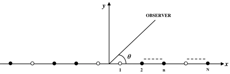
The radiating elements in the array of present interest are considered to be point sources spaced d=λ/2 apart. A symmetric linear array is shown in Fig.2. Mathematically, the array factor of a 2N element array is given by [13].

Fig. 2. Geometry of 2N element symmetric linear array placed along the x-axis.

Here, k=wave number= 2π/λ, λ=wave length.

θ= angle between the line of observer and array axis

θ0= scan angle

(An, φn) =excitation of current for the nth element on either side of the array. d=spacing between the radiating elements.

The fitness function associated with this array is the maximum Side Lobe Level of its associated radiation field pattern to be minimized. The general form of the fitness function is given by

( )

(

)

(

( )

)

(

20log10 E θ maxEθ0

)

Max

Fitness= (2)

Max |E (θ0)|=|E (θ)| -π/2 ≤ θ≤ π/2, θ≠ 00

4. Results

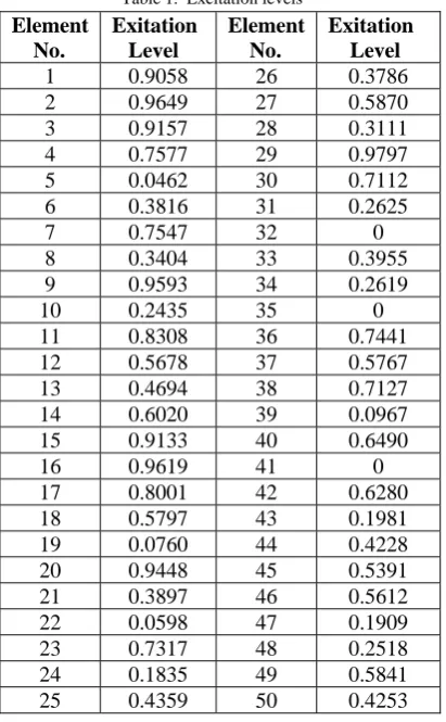
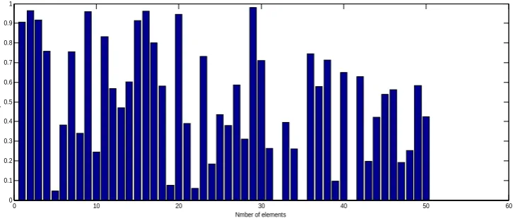
Results for optimizing the relative sidelobe level of a linear array of 100 elements are presented. Fig. 3. is shows the radiation pattern of an array of 100 point sources scanned to 00 after 50 iterations. The maximum relative sidelobe level is -40.98dB.Table 1 Lists the synthesized amplitude levels of the array. The amplitude levels of the half of the array are tabulated. Remaining array excitation levels are just mirror image of the right side because of the symmetry. The data from Table 1 is plotted as Fig.4 for additional clarity sake.

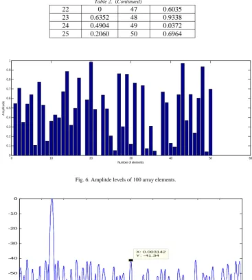
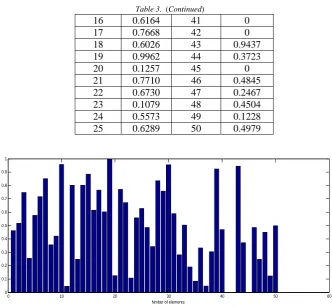
Computations are carried out to obtain the patterns of the array when the beam is steered to 450. Radiation pattern is shown in Fig. 5. The relative side lobe level observed is -40.66dB. The excitation levels are shown in Table 2. and these values are plotted in Fig. 6. The procedure is repeated to get the pattern at -450.The obtained radiation pattern is shown in Fig. 7.The side lobe level is -41.34 dB. The excitation levels for this scan angle are

x

y

θ

OBSERVER

(5)

tabulated in Table 3.and shown in Fig.8. In all the cases, the beam width calculated is same as for a uniform array of 100 elements.

-1 -0.8 -0.6 -0.4 -0.2 0 0.2 0.4 0.6 0.8 1 -60

-50 -40 -30 -20 -10 0

X: -0.3593 Y : -40.98

u

A

R

A

Y

F

A

C

T O

R

Fig. 3. Radiation pattern of 100 array elements at scan angle of 00

Table 1. Excitation levels Element

No.

Exitation Level

Element No.

1 0.9058 26 0.3786 2 0.9649 27 0.5870 3 0.9157 28 0.3111 4 0.7577 29 0.9797 5 0.0462 30 0.7112 6 0.3816 31 0.2625

7 0.7547 32 0

8 0.3404 33 0.3955 9 0.9593 34 0.2619

10 0.2435 35 0

11 0.8308 36 0.7441 12 0.5678 37 0.5767 13 0.4694 38 0.7127 14 0.6020 39 0.0967 15 0.9133 40 0.6490

16 0.9619 41 0

(6)

0 10 20 30 40 50 60 0

0.1 0.2 0.3 0.4 0.5 0.6 0.7 0.8 0.9 1

Nmber of elements

A

m

pli

tude

Fig. 4. Amplitude levels of 100 array elements at 00

-1 -0.8 -0.6 -0.4 -0.2 0 0.2 0.4 0.6 0.8 1

-60 -50 -40 -30 -20 -10 0

X: -0.2396 Y : -40.66

u

A

R

A

Y

F

A

C

T

O

R

Table 2. Excitation levels Element

No.

Element No.

1 0.5466 26 0.0521 2 0.7093 27 0.8589 3 0.3502 28 0.3013 4 0.5407 29 0.8541 5 0.6393 30 0.1182 6 0.1058 31 0.7640

7 0.7720 32 0

8 0.5303 33 0.7363 9 0.1500 34 0.0715 10 0.3592 35 0.3074 11 0.4243 36 0.0464

12 0.3968 37 0

13 0.6713 38 0.6679 14 0.8843 39 0.5567 15 0.3185 40 0.1279 16 0.4950 41 0.0885 17 0.8154 42 0.6407

18 0 43 0.9706

(7)

Table 2. (Continued)

22 0 47 0.6035

23 0.6352 48 0.9338 24 0.4904 49 0.0372 25 0.2060 50 0.6964

0 10 20 30 40 50 60

0 0.1 0.2 0.3 0.4 0.5 0.6 0.7 0.8 0.9 1

Number of elements

A

m

p

lit

u

d

e

Fig. 6. Amplitde levels of 100 array elements.

-1 -0.8 -0.6 -0.4 -0.2 0 0.2 0.4 0.6 0.8 1

-60 -50 -40 -30 -20 -10 0

X: 0.003142 Y : -41.34

u

A

R

A

Y

F

A

C

T

O

R

Table 3.Excitation levels Element

No.

Element No.

(8)

Table 3. (Continued)

16 0.6164 41 0

17 0.7668 42 0

18 0.6026 43 0.9437 19 0.9962 44 0.3723

20 0.1257 45 0

21 0.7710 46 0.4845 22 0.6730 47 0.2467 23 0.1079 48 0.4504 24 0.5573 49 0.1228 25 0.6289 50 0.4979

0 10 20 30 40 50 60

0 0.1 0.2 0.3 0.4 0.5 0.6 0.7 0.8 0.9 1

Nmber of elements

A

m

pli

tde

Fig. 8. Amplitde levels of 100 array elements.

Conclusion

It is evident from the results presented, this side lobe level is reduced from -13.5dB to about -40Db. the results presented are accurate as they are obtained after testing for convergence. The patterns are found to converge after 50 iterations. The beam width remains unaltered even after reducing the first side lobe level. However it has become necessary to compromise the rise in other side lobe levels.

References

[1] G. S. N. Raju, Antennas and Propagation, Pearson Education, 2005.

[2] C. A. Balanis, Antenna Theory Analysis and Design, 2nd_{Edition, John Willy & sons Inc, New York, 1997..}

[3] D. Mandal, S. K. Ghoshal, S. Das, S. Bhattacharjee, A. K. Bhattacharjee, Improvement of radiation pattern for linear array antennas using Genetic algorithm, International conference on recent trends in Information, telecommunication and computing, 2010. [4] C. L. Dolph, A current distribution for broad side arrays which optimizes the relationship between beamwidth and sidelobe level, Proc.., IRE 34:335-348, June, 1946.

[5] T. T. Taylor, Design of line source antennas for narrow beamwidth and side lobes, Proc.., IRE AP Trans 4:16-28(Jan 1955). [6] R. S. Elliot, Antenna theory and design, prentice-hall, New York, 1981.

[7] M. Shtimizu, Determining the Excitation coefficients of an array using genetic Algorithms, IEEE AP-S International Symposium: Seattle, June 19-24 1994, vol 1, pp.530-533.

[8] A. Tennant, M. Dawound, A. Anderson, Array pattern nulling by element position perturbations using a genetic algorithm, Electronic Letters, 3rd_{Febrary 1994, vol 30, No. 3, pp. 174-176.}

[9] J. Johnson, Y. Rahat-samaii, Genetic algorithm optimisation and its application to antenna design, IEEE AP-S International Symposium: Seattle, June 19-24 1994, vol. 1, pp. 326-329.

[10] R. L. Haupt, An Introduction to Genetic Algorithm for Electromagnetics, IEEE AP Magazine, April 1995 vol. 37, No. 2, pp 7-15. [11] R. L. Haupt, D. H. Werner, Genetic algorithms in Electromagnetics, Wiley- Interscience, IEEE Press, 2007

[12] B. P. Ng, M. H. Er, C. Kot, Linear array geometry synthesis with minimum sidelobe level and null control, IEE proc.,Microwave & Antennas Propag., June 1994, Vol. 141, No. 3.