R E S E A R C H
Open Access
Surface structure feature matching
algorithm for cardiac motion estimation
Zhengrui Zhang
1, Xuan Yang
2*, Cong Tan
2, Wei Guo
2and Guoliang Chen
2FromIEEE BIBM International Conference on Bioinformatics & Biomedicine (BIBM) 2016 Shenzhen, China. 15-18 December 2016
Abstract
Background: Cardiac diseases represent the leading cause of sudden death worldwide. During the development of cardiac diseases, the left ventricle (LV) changes obviously in structure and function. LV motion estimation plays an important role for diagnosis and treatment of cardiac diseases. To estimate LV motion accurately for cine magnetic resonance (MR) cardiac images, we develop an algorithm by combining point set matching with surface structure features of myocardium.
Methods: The structure features of myocardial wall are described by estimating the normal directions of points locating on the myocardium contours using an approximation approach. The Gaussian mixture model (GMM) of structure features is used to represent LV structure feature distribution. A new cost function is defined to represent the differences between two Gaussian mixture models, which are the GMM of structure features and the GMM of
positions of two point sets. To optimize the cost function, its gradient is derived to use the Quasi-Newton (QN). Furthermore, to resolve the dis-convergence issue of Quasi-Newton for high-dimensional parameter space, Stochastic Gradient Descent (SGD) is used and SGD gradient is derived. Finally, the new cost function is solved by optimization combining SGD with QN. With the closed form expression of gradient, this paper provided a computationally efficient registration algorithm.
Results: Three public datasets are employed to verify the performance of our algorithm, including cardiac MR image sequences acquired from 33 subjects, 14 inter-subject heart cases, and the data obtained in MICCAI 2009s 3D Segmentation Challenge for Clinical Applications. We compare our results with those of the other point set
registration methods for LV motion estimation. The obtained results demonstrate that our algorithm shows inherent statistical robustness, due to the combination of SGD and Quasi-Newton optimization. Furthermore, our method is shown to outperform other point set matching methods in the registration accuracy.
Conclusions: We provide a novel effective algorithm for cardiac motion estimation by introducing LV surface structure feature to point set matching. A new cost function is defined to measure the discrepancy between GMMs of two point sets. The GMM of point positions and the GMM of surface structure descriptor are defined at the same time. Optimization by combining SGD and Quasi-Newton is performed to solve the cost function. We experimentally demonstrate that our algorithm shows improved registration accuracy, and is convergent when used in high-dimensional parameter space.
Keywords: Gaussian mixture model, Surface structure feature, Point set matching, Stochastic gradient descent
*Correspondence: [email protected]
2College of Computer Science and Software Engineering, Shenzhen University, 518060 Shenzhen, China
Full list of author information is available at the end of the article
Background
Cardiovascular diseases (CVDs) are the leading cause of death in the developed world, as reported by the World Health Organization. Detecting the abnormalities in myocardial functions can assist the establishment of the early diagnosis of cardiomyopathy. The LV changes in structure and function during the development of cardio-vascular diseases. Analysis of LV structure using imaging instrument is shown to be effective in reducing CVDs mortality and morbidity. Magnetic Resonance Imaging (MRI) is a state-of-the-art technique for the direct exam-ination of changes in myocardial structure [1], with good spatial resolution and high signal to noise ratio. It allows the analysis of the structure alterations of LV and can be used to measure the functional change of LV.
Image registration technique can be employed to esti-mate LV motion for MR images, assisting the diagnosis of cardiac diseases [2, 3]. For instance, the myocardial hyper-trophy disease can be diagnosed by detecting parameters such as blood flow, ejection fraction, stroke volume, and so on [4]. Additionally, this technique allows the investi-gation of cardiac pathology as well.
A large number of methods for cardiac functional and motion modeling have been developed. At present, the methods of LV motion estimation can be classified into three groups: image intensity-based, geometrical and seg-mentation model-based, and point set matching-based.
Image intensity-based registration method optimizes a similarity function between images at different phases. A spatial transformation is used to compute the dis-placement of the myocardium [5, 6]. Chandrashekara et al. [7] used normalized mutual information between the short-axis and long-axis images to recover the complete three-dimensional motion of the myocardium. Ebrahimi et al. [8] introduced and evaluated the performance of a non-rigid joint multi-level image registration and intensity correction algorithm, which integrated inten-sity change compensation and motion correction into a unified model. Furthermore, Oubel et al. [9] applied an information-theoretic metric to measure the similar-ity between frames of tMRI for heart motion estimation. Shi et al. [10] used a spatially weighted similarity mea-sure between the untagged cine and the four-dimensional pseudo-anatomical MR image over time for myocardial motion estimation, while Bai et al. [11] combined the similarity metric between two images and the similarity between two probabilistic label maps of images to register atlases and segment cardiac MR datasets.
The geometrical and segmentation model-based meth-ods segment the myocardial wall and use active contours or surfaces to model the geometrical and mechanical structure of heart. In this model, geometric features are tracked to derive the motion of the heart walls and the dense displacement field was extracted by a
non-registration model [12]. Escalanteramírez et al. [13] estimated the motion of the heart based on the opti-cal flow and image structure information that was extracted from the steered Hermite transform coeffi-cients in sequential computed-tomography (CT) images. Papademetris et al. [12] segmented MR images and used a shape-tracking approach to establish correspondence of objects. Macan et al. [14] segmented the LV and extracted characteristic boundary points by investigating curva-ture distribution along the three-dimensional surface of cardiac wall. Points in two consecutive frames were matched by comparing curvature for LV motion estima-tion. Shi et al. [15] represented the LV surface shape using Delaunay triangulation and established correspondence between surface features to recover dense field motion from the tagged MR data.
The point set matching-based method is a type of feature-based registration method. Mathematically, point set matching can be represented as a problem to establish the point-to-point correspondence and the spatial trans-formation between two point sets at the same time. A cost function is defined to measure the discrepancy between two point sets based on a transformation function. The optimal transformation parameters are obtained by opti-mizing cost function. The iterative closest point (ICP) method [16] is the most commonly used point match-ing method, which estimates the global transformation between two point sets. ICP supposes a one-to-one cor-respondence between two point sets based on the nearest neighbor criterion, and estimate an affine transformation between two point sets. Algorithms were subsequently developed [17–19] to deal with elastic matching between two point sets based on the idea of ICP. Chui et al. [17] presented the point matching problem as a joint optimiza-tion problem over the parameterizaoptimiza-tion of the elastic spa-tial mapping and the softassign for the correspondence. However, the transformation estimated by [17] was based on the correspondence relationship between a virtual point set and a real point set, instead of correspondence relationship between two real point sets. This model was extended by Lin et al. [20], who used free-form defor-mation model in robust point matching to analyze LV motion. The FFD model was based on arbitrarily-shaped lattices instead of parallelepipedically-shaped lattices.
estimation of 3D echo images of LV. Liu et al. [21] defined a novel, more accurate and meaningful equivalent dis-tance to measure the position discrepancy between two point sets. Ravikumar et al. [22] proposed a probabilistic framework for group-wise rigid alignment of point-sets using a mixture of Student’s t-distribution. Their method reduces alignment errors significantly in the presence of outliers. Du et al. [23] integrated a Gaussian probability model into the bounded-scaled registration problem to deal with the alignment of point sets with noise.
Here, we employ point set matching-based method to estimate motion of LV. Considering that existed point set matching methods are primarily based on the spa-tial relationship between two point sets, we introduce the structure information of LV to point set matching to improve LV registration accuracy at different time points. In this study, we develop a novel point set match-ing algorithm by considermatch-ing the surface structure of LV. The key contributions of this study are as follows: (1) The normal direction is computed as the surface struc-ture feastruc-ture to describe the strucstruc-ture of myocardial wall. Additionally, a cost function for the determination of the discrepancy of the GMMs of positions and GMMs of surface structures of two point sets is developed. (2) To resolve the dis-convergence problem of the optimization in high-dimensional parameter space, the Stochastic Gra-dient Descent (SGD) is combined with Quasi-Newton method in order to estimate optimal transformation parameters.
Methods
Overview of the methodology
Two cardiac slices taken at different times are consid-ered a target image and a source image. For example, the slice obtained in the end-diastole represent a target image and the one obtained in end-systole represent the source image. Point sets are extracted from these images, and the point set in the target image is considered a scene set, while the other represent a model set. Since the slice num-bers of two 3D cardiac images along long axis are different, we interpolate the point sets along this axis to obtain an equal number of slices of two corresponding 3D cardiac images. Afterwards, corresponding slices are considered source image and target image. The surface structure fea-tures of points located on myocardial wall are estimated approximately. A new cost function is defined as the com-bination of the GMM of spatial locations and the GMM of surface structures between two point sets, which is optimized by SGD and Quasi-Newton methods.
Point interpolation along the long axis
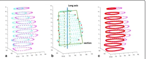
Cardiac MR spatial resolution is low along the long axis and relatively high along the short axis, as shown in Fig. 1. Moreover, slice numbers of two 3D cardiac MR images in
Fig. 1A MR cardiac image:a3D heart image after scaling along z axis; ba slice of the 3D image along z axis
different phases differ. Two point sets in end-systole and end-diastole phases are illustrated slice by slice in Fig. 2a respectively, which demonstrates that the slices in these two images do not matched each other along the long axis. To resolve this problem, points are interpolated along long axis to equalize the number of slices between two images. Next, point sets of the corresponding slices are registered. To interpolate point sets along the long axis, we con-struct a section traversing the center of LV image and being parallel to the long axis, as shown in Fig. 2b. All the points of this section are interpolated. At first, the original point sets are interpolated by B-spline interpolation on the
xyplane slice by slice to ensure that there are dense sam-pled points on the section. For a given section, all points located on the section are interpolated to make the slice numbers of two 3D point sets to be equal. Secondly, the section is rotated around the long axis to obtain a new section, and the point interpolation on the new section is performed again. Repeating the described procedure, we obtain a number of points along the long axis and make sure that the number of slices in two 3D LV images are equal. Figure 2c shows an example of an interpolated point set, where red points represent the interpolated points.
Surface structure description
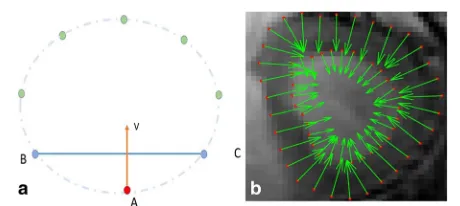
The heart is composed of a muscular contractile organ (myocardium) surrounded by two layers of connective tis-sue, endocardium and epicardium. The LV and right ven-tricle (RV) are separated by endocardium and epicardium. The cardiac LV has a thick muscular wall, and its struc-ture can be approximated by a curved surface. Here, we describe the curved surface of myocardial wall using structure features, described by the normal directions of points located on the myocardial wall. Fig. 3a shows the extracted points from a slice, andBandCare two points nearest to pointA. As we know, a point with tangential direction −→BC exists based on the Lagrange mean value theorem. The normal direction ofAcan be approximated as the perpendicular line to−→BCwhenBandCare close to
Aenough. That implies, dense sampled points can ensure the accuracy of this approximation. An example of normal direction estimation is presented in Fig. 3b.
Let S = (s1,s2, ...sn)T be the scene point set with n
points, and M0 =
m01,m02, ...m0mT be the model point set with m points, where si,i = 1, 2, ...,n and m0j,j =
1, 2, ...,mare two dimensional points. Supposingsiandsj
are the nearest two points ofsk, the normal direction
vec-tor ofsk can be represented asvk = Hk
0 −1
1 0
, where
Hk = sj − si. Then, the surface structure description VS=[v1,· · ·,vn]T of scene point set can be presented as
VS=[H1H2...Hn]T
0 −1 1 0
. (1)
For the model point set M0, we denote its mapped
point set asM= (m1,m2, ...,mm)under a spatial
trans-formation. Following this, we will describe the surface structure descriptionVMofM. Here, we employ the thin
plate splines (TPS) to be the spatial transformation. Let
Q=q1,q2, ...,qc be the control point sets withcpoints, qj =
qjx,qjy
, j = 1,· · ·,c. The mapped model point
mi =
mix,miy
, i = 1,· · ·,m, is expressed by TPS as
Fig. 3Illustration of the normal directions of points.aBandCare two points nearest toA; approximated normal direction perpendicular to the line crossBandC;bnormal directions of points
follows:
mix=a0x+a1xm0ix+a2xm0iy+ c
j=1 wjxφ
m0i−qj
miy=a0y+a1ym0ix+a2ym0iy+ c
j=1
wjyφm0i−qj,
(2)
whereφ(r)= −r2log(r2)is the TPS basis function in 2D; m0i−qjis the Euclidean distance betweenm0i andqj;a0x, a1x,a2xare affine coefficients;wjxandwjy,j=1,· · ·,c, are
elastic coefficients inxandyaxes respectively. The Eq. (2) can be rewritten as:
M=[ 1|M0]A+W, A=
⎡ ⎣aa01xx aa01yy
a2x a2y
⎤
⎦, (3)
[ 1|M0]=
⎡ ⎢ ⎢ ⎣
1 m01x m01x
1 m02x m02x
1 . . . . 1 m0
mx m0mx
⎤ ⎥ ⎥
⎦,W=
⎡ ⎢ ⎢ ⎣
w1x w1y w2x w2y
. . . .
wcx wcy
⎤ ⎥ ⎥ ⎦.
where [1|M0] is am×3 matrix;Ais a 3×2 matrix;Wis
ac×2 matrix.isn×cmatrix withφij=φm0i −qj.
LetNbe the left null space of [1|Q], which is ac×(c−3) matrix. A new(c−3)×2 matrixτ is defined by satisfying
W=Nτ, which is used to represent the elastic parame-ter. The transformation parameter θ contains the affine parameterAand elastic parameterW, which can be rede-fined asθ=[ANτ]. Then, the mapped model point setM
is related to the model setM0as
M=[1|M0N]θ. (4)
Assumingmi andmjare the nearest two points ofmk,
the normal direction ofmkcan be approximated asuk=
(mj−mi)
0 −1 1 0
. Based on above analysis, it is known
mi =[ 1|M0 N]iθ, where [ 1|M0N]i is theith row of
the matrix [ 1|M0 N]. We denote Bi as [ 1|M0 N]i,
and the normal direction ofmkcan be expressed asuk= Tkθ
0−1 1 0
, whereTk = Bj−Bi. Therefore, the surface
structure descriptionVM=[u1,· · ·,um]T of the mapped
model point set under parametersθis
VM=[T1T2...Tm]Tθ
0 −1 1 0
. (5)
Point set matching using GMMs
two Gaussian mixtures to align two point sets. In [19], they describe the gaussian mixture density function as accumulation of k gaussian functions,
p(x)=ki=1αiφ(x|μi,σi),ki=1αi=1, whereφ(x|μi,σi)
is a gaussian function with mean vectorμiand varianceσi.
As we know, when the number of Gaussian model is large enough, almost any probability density can be well approximated by this model. The GMM of the point setM
can be represented as a gaussian mixture density function as:
gmm(x,M)= 1 m
m
i=1
1
√
2πσexp
−1
2(x−mi)
Tσ−1(x−m i)
.
(6)
In this model, all variances are same toσ; each pointmi
inMis the mean of theith gaussian function.
In the method presented by Bingjian et al. [19], only spatial information is employed for point set matching, instead of introducing additional information, such as the object structure. Surface structure description is a kind of structure features to represent the anatomical structure of LV myocardial wall. Following this, we improve point set matching accuracy by introducing the surface structure feature to the gaussian mixture density. Based on a previ-ous study [19], we expand the point set matching model by introducing the discrepancy of the GMM of surface structure features.
Similar to the GMM of point positions, the GMM of surface structure features ofVMis defined asgmm(v,VM),
where v and VM are similar to x and M in (6). We
selectL2distance to determine the similarity between two Gaussian mixtures of surface structure descriptions, then the discrepancy between two GMMs of surface structure features is(gmm(v,VM)−gmm(v,VS))2dv. Putting the
discrepancy of all GMMs together, a new cost function of point set matching is defined as,
dL2(S,M,VS,VM)=
(gmm(x,M)−gmm(x,S))2dx
+β
(gmm(v,VM)−gmm(v,VS))2dv+λ
2trace(W
TKW).
(7)
The first term in Eq. (7) is the discrepancy of GMMs based on point positions, and the second term is the discrepancy of GMMs based on surface structure descrip-tions of point sets. λ2WTKWis a penalty term to regular-ize the transformation to be smooth, where theijth entry of matrixKisKij=φ(qi−qj),i,j=1,. . .,c.λandβare
coefficients to balance the terms in Eq. (7). For LV motion estimation, the model setM0is extracted from the end-systole (ES) phase and the scene setSis extracted from the end-diastole (ED) phase. The goal of LV motion estima-tion is to find the parameterθ of a spatial transformation by minimizing the cost function (7).
The Eq. (7) can be rewritten as:
dL2(S,M,VS,VM)=
(gmm(x,M))2dx
−2
gmm(x,M)gmm(x,S)dx+
(gmm(x,S))2dx
+λ
2trace(W
TKW)+β(gmm(v,VS))2dv
−2β
gmm(v,VM)gmm(v,VS)dv+β
(gmm(v,VM))2dv,
(8)
The closed-form expression between two gaussian mix-tures can be easily derived as:
gmm(M)gmm(S)dx= 1 mn
m
i=1 n
j=1 exp
−(mi−sj)2
σ2
,
(9)
based on the following formula:
φ(x|μ1,σ1)φ(x|μ2,σ2)dx=φ(0|μ1−μ2,σ1+σ2), (10)
Following this, Eq. (8) can be formulated in detail,
dL2(S,M,VS,VM)=
1
m2 m
i=1 m
j=1 exp
−mi−mj2
σ2 − 2 mn m
i=1 n
j=1 exp
−miσ−2sj2
+ 1 n2
n
i=1 n
j=1 exp
−si−σ2sj2
+λ
2trace
WTKW
+ β m2
m
i=1 m
j=1 exp
−ui−uj2
σ2
−2β mn
m
i=1 n
j=1 exp
−ui−vj2
σ2 +β n2 n
i=1 n
j=1 exp
−vi−σ2vj2
,
(11)
Removing irrelevant terms in Eq. (11), the final cost functionJis:
J= 1 m
m
i=1
⎧ ⎨ ⎩ 1 m m
j=1 exp
−mi−σ2mj2
−2 n
n
j=1 exp
−mi−sj2
σ2 +β m m
j=1 exp
−ui−uj2
σ2
−2β n
n
j=1 exp
−ui−vj2
σ2 ⎫⎬ ⎭+ λ 2trace
WTKW
,
It is noteworthy thatJ is convex and is differentiable, which implies that gradient-based optimization tech-niques can be used to optimize J, such as the Quasi-Newton method.
Optimization using the Quasi-Newton method
Quasi-Newton method represents one of the most effec-tive ways to solve the nonlinear optimization problem, with fast convergence speed and high accuracy. Here, we derive the gradient of Eq. (12) in detail. We seperateJas
J =Jd+Jv, whereJdis the sum of the first two items and
λ
2WTKW, andJvrepresents the other two items.
Jd=
1
m m
i=1
⎧ ⎨ ⎩ 1 m m
j=1 exp
−mi−σ2mj2
(13) −2 n n
j=1 exp
−mi−sj2
σ2 ⎫⎬ ⎭+ λ 2trace
WTKW
,
Jv=
1
m m
i=1
⎧ ⎨ ⎩ β m m
j=1 exp
−ui−uj2
σ2
(14)
−2β n
n
j=1 exp
−ui−vj2
σ2
⎫⎬
⎭,
Then,
∂Jd
∂θ =
$∂Jd ∂A
∂Jd ∂τ
%
=
[ 1|M0]TG
(N)TG+λNTKNτ
, (15)
where G= ∂∂MJ is am× 2 matrix. Jv can be written as Jv=mβ2J1,v−mn2βJ2,v, where
J1,v= m
i=1 m
j=1 exp
−ui−uj2
σ2
J2,v= m
i=1 n
j=1 exp
−ui−σ2vj2
.
(16)
Obtaining the derivatives ofJ1,vandJ2,vis simple:
∂J1,v ∂θ =
m
i=1
m
j=1
exp
−ui−σ2uj2
·
−2
Ti−Tj T
Ti−Tj θ σ2 , (17)
∂J2,v
∂θ =
m
i=1 n
j=1 exp
−ui−σ2vj2
·
−2TiT
Tiθ−Hj
σ2
.
(18)
Therefore, the derivatives ofJvcan be obtained as
∂Jv
∂θ = β
m2
∂J1,v
∂θ −
2β
mn
∂J2,v
∂θ , (19)
while the derivatives of Eq. (12) can be obtained as
∂J
∂θ = ∂Jd
∂θ + ∂Jv
∂θ, (20)
Although Quasi-Newton method can solve the non-linear optimization problem, it might be divergent in high dimensional parameter space. In other word, Quasi-Newton method cannot possibly find solutions when there are too many control points. In order to resolve this issue, the Stochastic Gradient Descent (SGD) algorithm is employed to optimize Eq. (12) robustly. Furthermore, considering that using SGD is not good at obtaining the precise solution, Quasi-Newton method is performed fur-ther to improve the accuracy of solution when SGD is convergent.
Optimization using Stochastic Gradient Descent
Quasi-Newton method uses the full training set to update parameters at each iteration, which tends to converge to local optima easily in high dimensional parameter space. SGD addresses this issues by following the negative gradient of the cost function using only a single or a few training examples [25]. By measuring gradient changes, it is easy to construct a model of the cost function to produce a superlinear convergence. SGD can follow the negative gradient of the cost function after being exposed to only a single or a few training examples, which can overcome computation cost and lead to fast convergence. Observing that our cost function defined above is dif-ferentiable, the SGD algorithm can simply compute the gradient of the cost function using only a single mov-ing model pointmi. Let f(θ,i)be the part ofJ, which is
influenced bymi:
f(θ,i)= 1 m
m
j=1 exp
−mi−σ2mj2
−2 n
n
j=1 exp
−mi−sj2
σ2
+λ
2trace
WTKW
+β m
m
j=1 exp
−ui−uj2
σ2
−2β n
n
j=1 exp
−ui−vj2
σ2
The five terms in Eq. (21) are denoted asf1,f2,f3,f4,f5,
respectively. Then, the derivatives of f(θ,i) is ∂f∂θ(θ,i)
= ∂f1
∂θ + ∂∂θf2+∂∂θf3+∂∂θf4+∂∂θf5. The derivative of each term is:
∂f1
∂θ =
1
m
⎧ ⎨ ⎩BiT·
m
j=1 exp
−mi−σ2mj2
·
&
−σ22
'
·(mi−mj)
+ m
j=1 BjT·
2
σ2·exp
−mi−mj2
σ2
·(mi−mj)
⎫ ⎬ ⎭,
∂f2
∂θ =−
2
n·Bi T·
n
j=1 exp
−miσ−2sj2
·
&
−σ22
'
·(mi−sj),
∂f3
∂θ = λ
2
03∗22NTKNτ
T
,
∂f4
∂θ = β
m m
j=1 exp
−ui−σ2uj2
·
−2(Ti−Tj)σT2(Ti−Tj)θ
,
∂f5
∂θ =−
2β
n n
j=1 exp
−ui−σ2vj2
·
−2TiT(Tσi2θ−Hj)
, (22)
Based on the SGD procedure, Algorithm 1 represents details of optimization using SGD.
Algorithm 1Point set matching using SGD method
Input: the model setM0, the scene setS, an initial
param-etersθand learning rateη;
1: repeat
2: Compute the moving model point setMusingθ. 3: Shuffle points inMrandomly.
4: for i=1, 2, ...,mdo
5: θ:=θ−η·∂f∂θ(θ,i);
6: end for
7: Update the learning rateη.
8: untilan approximate minimum is obtained
SGD algorithm is robust to obtain an approximate solu-tion, but it is not good at finding an accurate solution. To improve the solution accuracy further, Quasi-Newton method is employed for the optimization of Eq. (12), beginning at the optimal solution obtained by SGD.
Results and discussion
In order to confirm the improved performance of our method, three cardiac datasets are used. The first dataset included cardiac MR image sequences acquired from 33 subjects [26], the second set is composed of 14 inter-subject heart slices [27], while the third set is the MIC-CAI 2009s 3D Cardiac Segmentation Challenge dataset [28]. In our study, the Quasi-Newton method and the
combination of SGD and Quasi-Newton method are employed to demonstrate the improved performance of optimization of the cost function. The name following “SSD" in this article represents the optimization used in our method, and for example, “SSD_QN" denotes that the Quasi-Newton method is used. To compare the per-formance of our method with those of the previously developed methods, GMM [19] and CPD [18] methods are evaluated as well.
Cardiac MR image registration
Initially, we use a cardiac dataset [26] to evaluate the regis-tration accuracy of our method. In this dataset, 33 cardiac MR image sequences are provided. Each image sequence consisted of 20 frames and the number of slices acquired along the long axis ranged from 8 to 15. The distance between slices ranged from 6 to 13mm. The size of all image slices is 256× 256 pixels with a pixel-spacing of 0.93-1.64mm[26].
We evaluate the registration accuracy of our algo-rithm by registering cardiac images at the end-diastole phase and the end-systole phase. The point sets of LV at end-diastole and end-systole phases are regis-tered. Here, these points are provided by experts [26] in order to eliminate the effects of cardiac segmenta-tion. The point set at end-diastole phase is the scene point set, and the one at end-systole phase is the model point set. The end-systole points are interpo-lated along the long axis to make the slice numbers equal to that in the end-diastole points. Afterwards, these two point sets are matched using our algorithm slice by slice. In Fig. 4, the interpolated model points and scene points are presented, and they are extracted from the slices in end-systole and end-diastole phases respectively.
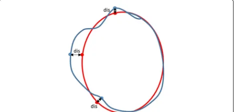
Average Perpendicular Distance (APD) between the mapped model point set and the scene point set is com-puted to evaluate our algorithm quantitatively. The APD
represent the average distance between two point sets, as shown in Fig. 5.
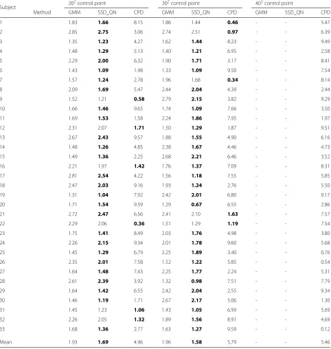
We use 102control points to estimate the transforma-tion functransforma-tion between end-systole and end-diastole slices. Table 1 lists the APD results of 33 subjects using three different algorithms. For each subject, the APD is aver-aged registered results of all corresponding slices along the long axis. Noted that the APD results of SSD_QN are smaller than that of GMM and CPD for most subjects. It implies that the registration accuracy can be improved by introducing the surface structure features to the point set matching.
Analyses conducted using the Quasi-Newton method demonstrate the issue of divergence that appears with large number of control points. We increase the number of control points from 202to 402. The APD results are
listed in Table 2, and we show that the results obtained by applying the SSD_QN and GMM methods diverge when too many control points used, while CPD is shown to be robust in convergence. For the convergent SSD_QN, it outperforms GMM and CPD in respect of APD for most cases.
To demonstrate the improved performance of SSD_S -GD_QN further, 502 control points are used to regis-ter the slices between end-systole and end-diastole in all samples. In Fig. 6, APD results obtained for 33 subjects using CPD and SSD_SGD_QN with 502 control points are presented. Since GMM is divergent, the APD results obtained by this method are not provided in Fig. 6. For the majority of cases, SSD_SGD_QN outperforms CPD, which demonstrates the stability of SSD_SGD_QN in high dimensional parameter space.
Registration of the inter-subject LV
Furthermore, we use a cardiac dataset provided by the Danish Research Centre for Magnetic Resonance (DRCMR) [27], comprising 14 gray scale 256 × 256 images. All images used are short-axis, end-diastolic car-diac MR images, acquired using a whole-body MR unit
Fig. 5APD schematic diagram. The red point set is the ground truth and the sky blue point set is the mapped model set. Thedisis minimum vertical distance between two point sets
Table 1The APD (∗10−2mm) results of 33 subjects using three methods
Cases SSD_QN GMM CPD
1 1.65 1.55 5.35
2 2.53 2.36 1.07
3 2.22 1.94 6.85
4 2.31 2.17 2.58
5 2.08 1.89 1.71
6 2.05 1.96 1.35
7 1.91 1.88 1.14
8 2.05 1.89 9.74
9 2.72 2.63 6.96
10 1.88 1.67 2.07
11 1.75 1.69 8.03
12 1.98 1.84 1.55
13 2.85 2.61 5.57
14 2.45 2.26 1.32
15 2.16 2.01 4.86
16 2.42 2.29 4.23
17 1.50 1.32 1.98
18 2.39 2.21 2.22
19 2.68 2.46 1.97
20 1.47 1.36 1.93
21 1.64 1.46 6.72
22 1.94 1.84 9.37
23 1.79 1.59 2.14
24 2.34 2.17 6.23
25 1.92 1.74 9.37
26 1.59 1.44 6.72
27 2.86 2.73 5.13
28 1.54 1.35 1.22
29 2.83 2.71 9.71
30 2.70 2.52 4.60
31 1.95 1.79 5.12
32 1.84 1.57 4.71
33 2.78 2.66 6.33
Mean 2.14 1.99 4.54
(The bold one is the optimal result)
(Siemens Impact) operating at 1.0 Tesla. The endocardial and epicardial contours of the LV are manually annotated by experts [27].
Table 2The APD (∗10−2mm) results of 33 subjects using three methods with different number of control points
Subject 20
2control point 302control point 402control point
Method GMM SSD_QN CPD GMM SSD_QN CPD GMM SSD_QN CPD
1 1.83 1.66 8.15 1.86 1.44 0.46 - - 5.47
2 2.85 2.75 3.06 2.74 2.51 0.97 - - 6.39
3 1.35 1.23 4.27 1.62 1.44 8.23 - - 9.49
4 1.48 1.29 5.13 1.40 1.21 6.95 - - 2.58
5 2.29 2.00 6.32 1.90 1.71 3.17 - - 8.41
6 1.43 1.09 1.98 1.33 1.09 9.50 - - 7.54
7 1.57 1.24 2.78 1.96 1.68 0.34 - - 8.14
8 2.09 1.69 5.47 2.44 2.04 4.39 - - 2.44
9 1.52 1.21 0.58 2.79 2.15 3.82 - - 9.29
10 1.66 1.46 9.65 1.74 1.09 7.66 - - 3.50
11 1.69 1.53 1.58 2.24 1.86 7.95 - - 1.97
12 2.31 2.07 1.71 1.50 1.29 1.87 - - 9.51
13 2.67 2.43 9.57 1.88 1.55 4.90 - - 6.16
14 1.48 1.26 4.85 2.38 1.67 4.46 - - 4.73
15 1.49 1.36 2.25 2.68 2.21 6.46 - - 3.52
16 2.21 1.97 1.42 1.76 1.37 7.09 - - 8.31
17 2.81 2.54 4.22 1.56 1.18 7.55 - - 5.85
18 2.47 2.03 9.16 1.93 1.24 2.76 - - 5.50
19 1.31 1.04 7.92 2.42 2.01 6.80 - - 9.17
20 1.71 1.54 9.59 1.29 0.67 6.55 - - 2.86
21 2.72 2.47 6.56 2.41 2.10 1.63 - - 7.57
22 2.29 2.06 0.36 1.51 1.29 1.19 - - 7.54
23 1.75 1.41 8.49 2.03 1.76 4.98 - - 3.80
24 2.26 2.15 9.34 2.01 1.78 9.60 - - 5.68
25 1.45 1.29 6.79 2.25 1.89 3.40 - - 0.76
26 2.35 2.01 7.58 1.52 1.22 5.85 - - 0.54
27 1.64 1.48 7.43 2.25 1.77 2.24 - - 5.31
28 2.61 2.39 3.92 1.32 0.98 7.51 - - 7.79
29 1.64 1.42 6.55 2.42 2.04 2.55 - - 9.34
30 1.46 1.19 1.71 2.67 2.17 5.06 - - 1.30
31 1.45 1.23 1.06 1.43 1.05 6.99 - - 5.69
32 2.26 2.05 1.32 1.89 1.56 8.91 - - 4.69
33 1.68 1.36 2.77 1.63 1.27 9.59 - - 0.12
Mean 1.93 1.69 4.96 1.96 1.58 5.79 - - 5.46
(The bold one is the optimal result, and ‘-’ denotes divergence)
contour marked by an expert, to evaluate the registration accuracy. We use the APD to evaluate the performance of three methods, since it can be used to evaluate the registration accuracy of three methods.
We locate the region of interest (ROI) in heart in the original image, and employ the template matching [29] algorithm (TMA) to extract epicardium and endocardium profiles by constructing many typical LV templates.
The candidate template is generated by a particle, and the optimal particle is obtained by matching the target and the candidate templates. Following this, the point sets of epicardium and endocardium are extracted around the candidate template contour, as shown in Fig. 7.
In this experiment, 102control points are employed to
Fig. 6The APD results using SSD_SGD_QN and CPD respectively
and CPD in all cases except case 13. In this case, many noisy points are observed in the extracted myocardial contour, which leads to the registration errors.
To visualize the registration results further, we present the registration results obtained by three methods for case 2 in Fig. 8. The ground truth is marked by red points, and the mapped contours estimated by three methods are marked by green points. The outlines of endocardium and epicardium, obtained using SSD_QN, are shown to be close to the ground truth. Moreover, these outlines are demonstrated to be smoother than those obtained using GMM and CPD, which demonstrates the advantage of surface structure feature for the description of the circular structure of myocardium.
Furthermore, we use SSD_SGD_QN to demonstrate the optimization performance in point registration. In Fig. 9, the APD results obtained using SSD_SGD_QN, GMM, and CPD with 202control points are presented. Although GMM is shown to converge in this experiment, its reg-istration accuracy is not satisfactory. CPD is shown to be converged, but the APD results obtained using this method are shown to be larger than those determined using SSD_SGD_QN and GMM.
Registration of cine MR cardiac images
In order to confirm the superior performance of our method in the registration of cine MR cardiac images, we analyze 15 cardiac cine MR validation datasets from the
Fig. 7Extracted scene point set (a) and model point set (b)
Table 3The APD (∗pixel) results of inter-subject registration using three methods
Cases SSD_QN GMM CPD
2 1.07 1.16 1.20
3 0.79 0.87 1.19
4 1.32 1.38 1.82
5 1.80 1.94 1.85
6 1.56 1.66 1.74
7 1.45 1.49 1.73
8 1.08 1.25 1.67
9 1.66 1.71 1.69
10 1.57 1.71 1.82
11 1.42 1.45 1.59
12 0.73 0.84 1.04
13 1.84 1.80 1.93
14 1.85 1.94 1.89
Mean 1.39 1.48 1.63
Std 0.38 0.37 0.29
(The bold one is the optimal result)
MICCAI 2009s 3D Segmentation Challenge for Clinical Applications [28], provided by the Sunnybrook Health Sciences Centre. Cine steady state free precession (SSFP) MR short axis (SAX) images are obtained using 1.5T GE Signa MRI, during 10-15 s breath-holds with a tempo-ral resolution of 20 cardiac phases over the heart cycle, and scanned from the enddiastolic phase. Six to 12 SAX images are obtained from the atrioventricular ring to the apex (thickness = 8mm, gap = 8mm, FOV = 320mm×
320mm, matrix = 256×256) [28].
Fig. 9Comparison of APD using SSD_SGD_QN, GMM and CPD with 202control points for registration of inter-subject LV
This MR cardiac image dataset is used for MICCAI 2009s 3D Segmentation Challenge for Clinical Applica-tions. Cardiac image segmentation is related to the image registration, and the segmentation results of one slice obtained in a single time point can be propagated to other time points using deformable registration, which takes advantage of the strong temporal correlation between phases. Here, we analyze the transformation between slices at the enddiastolic and endsystolic phases. Reg-istrations are performed from enddiastole to endsystole and vice versa. The LV contours extracted from the endsystolic phase can be mapped to the enddiastolic phase using the estimated transformation, representing the segmented results of LV at enddiastole, and vice versa.
For this analysis, we eliminate the surrounding organs and locate the area containing LV. Considering that only the contour of endocardium is provided in MICCAI 2009s dataset, we segment the endocardium and extract the boundary points of endocardium by edge detection. We ignore the effects of the papillary muscles of endocardial wall, as they are minor. Since the outline of endocardium is irregular, we smooth out the border by using Savitzky-Golay polynomial filter [30]. The original cardiac slice and an automatically extracted endocardial outline are presented in Fig. 10.
Two principal evaluation standards in the MICCAI 2009s 3D Segmentation Challenge for Clinical Applica-tions are the APD, which measures the average distance
Fig. 10An example of endocardium contour extraction
Table 4The APD (∗mm) results of 15 subjects using three methods
Cases SSD_QN GMM CPD
SC-HF-I-05 1.42 1.40 1.45
SC-HF-I-06 1.30 1.36 1.35
SC-HF-I-07 2.90 2.90 3.06
SC-HF-I-08 1.44 1.55 1.60
SC-HF-NI-07 2.13 2.42 2.71
SC-HF-NI-11 1.16 1.27 1.22
SC-HF-NI-31 1.91 1.90 2.19
SC-HF-NI-33 2.16 2.22 2.46
SC-HYP-06 1.53 1.49 1.54
SC-HYP-07 2.83 2.84 3.01
SC-HYP-08 1.52 1.61 1.51
SC-HYP-37 1.80 1.42 1.34
SC-N-05 2.49 2.55 2.43
SC-N-06 2.51 2.46 2.58
SC-N-07 1.72 1.84 1.84
Mean 1.92 1.95 2.02
Std 0.56 0.57 0.64
(The bold one is the optimal result)
error between two point sets, and the Dice Metric (DM), that shows the contour overlap proportion between the mapped contour and the target contour. DM = 2S3
S1+S2,
where S1 andS2 are endocardial surface areas obtained
Table 5The DM results of 15 subjects using three methods
Cases SSD_QN GMM CPD
SC-HF-I-05 0.94 0.94 0.94
SC-HF-I-06 0.95 0.95 0.95
SC-HF-I-07 0.90 0.90 0.89
SC-HF-I-08 0.95 0.95 0.94
SC-HF-NI-07 0.93 0.92 0.92
SC-HF-NI-11 0.96 0.96 0.96
SC-HF-NI-31 0.93 0.93 0.92
SC-HF-NI-33 0.86 0.86 0.85
SC-HYP-06 0.90 0.91 0.90
SC-HYP-07 0.80 0.80 0.79
SC-HYP-08 0.93 0.93 0.93
SC-HYP-37 0.85 0.88 0.89
SC-N-05 0.77 0.77 0.77
SC-N-06 0.85 0.85 0.85
SC-N-07 0.92 0.92 0.92
Mean 0.90 0.90 0.89
Std 0.06 0.06 0.06
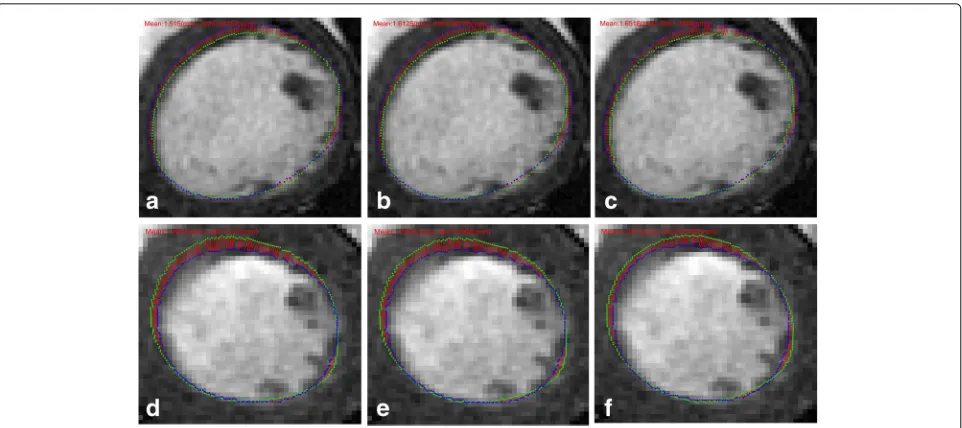
Fig. 11Illustration of APD using three methods for case SC-HF-I-05. From left to right: SSD_QN, GMM and CPD.a,bandcshow the registration results of an ES slice to the corresponding ED slice;d,eandfshow the registration results of an ED slice to the corresponding ES slice
manually by experts and by automatic methods, while
S3 represents the overlap area between S1 and S2. A
higher DM values indicates better registration results. The forward registration (endsystole to enddiastole) and the reverse registration (enddiastole to endsystole) are per-formed respectively. All these DM values represent the average of registration results in two directions.
We used 102control points to estimate the transforma-tion functransforma-tion between two heart slices, and 15 clinical cine MR cases with four patient categories (heart failure, with (HF-I) or without (HF-NI) ischemia, hypertrophy (HYP), and normal (N)) are used to investigate the performance of SSD_QN, GMM, and CPD.
In Tables 4 and 5, the APD and DM results obtained using three described methods are presented. The APD results obtained by SSD_QN are shown to be smaller than those obtained by GMM and CPD in most cases, except for one case. In the case of SC-HYP-37, the extracted points are not able to outline the endocardium wall, which led to the deviation of the normal direc-tions of points. Consequently, registration accuracy using SSD_QN decreased, which indicates that the initial seg-mentation results affect the precision of registration.
For a detailed illustration of the registration results, the mapped contour and the contour marked by experts using the data from subject SC-HF-I-05 are presented in Fig. 11. The first line shows the slices in the enddiastolic phase and the mapped endsystolic contours using SSD_QN, GMM, and CPD. The second line indicates the slices in the endsystolic phase and the mapped enddiastolic con-tours using three methods. The ground truths are marked
by green points, and the mapped contours are denoted by blue points. Short red lines illustrate the minimum distance between the points marked by the expert and the mapped points. The shortening of the red lines indi-cate a higher registration accuracy. The APD obtained by SSD_QN is shown to be superior to that obtained by GMM and CPD for forward registration. However, the APD of the reverse registration obtained using SSD_QN is larger than that obtained using GMM and CPD, because the parameters used in our experiments are suitable for forward, and not reverse registration.
The APD obtained by SSD_SGD_QN, GMM, and CPD with 202 control points are compared as well in Fig. 12. Similar to the previously presented results, GMM and CPD are converged with these parameters as well, and the APD obtained using SSD_SGD_QN is shown to be close to those obtained using GMM and CPD.
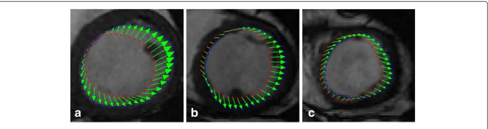
Fig. 13 a,bandcshow displacement vectors of different slices of ED for case SC-HF-I-05
Finally, the displacement vector graphs estimated by our algorithm SSD_QN with 102control points are illus-trated in Fig. 13. Displacement vectors of LV from endsys-tole to enddiasendsys-tole in three slices are shown, where red points and blue points represent the model and the mapped model points, and green arrows illustrate the displacement vectors of these points. The estimated LV motion is shown to coincide generally with the real motion.
Conclusion
LV motion estimation is important in quantitative assess-ment of myocardial function and dynamic behavior of human heart, which is invaluable in the diagnosis of cardiac diseases. In this paper, a novel point set match-ing algorithm is proposed to estimate LV motion. The main contribution of the proposed algorithm is introduc-ing the structure feature of LV to point set matchintroduc-ing. The surface structure features of LV is described using normal directions, and the GMM of surface structure features is defined. By measuring the discrepancy of all GMMs of two point sets, a new cost function of point set matching is constructed. SGD and Quasi-Newton method are combined to optimize the cost function. Performance of our algorithm is verified using three car-diac image datasets. The obtained results demonstrate that when small amount of control points used, our algorithm with Quasi-Newton optimization outperforms GMM and CPD in LV motion estimation. When too many control points used, our algorithm with the com-bination of SGD and QN optimization is more robust than GMM and CPD. The evaluation performed using MICCAI 2009s 3D Segmentation Challenge for Clinical Applications dataset demonstrate that the applicability of our motion estimation method remains the same when analyzing different cardiac diseases. The method we develop and present here could be applied to clinically-obtained data, to demonstrate its applicability in a clinical environment.
Abbreviations
APD: Average perpendicular distance; CPD: Coherent point drift; DM: Dice metric; GMM: Gaussian mixture model; Icp: Iterative closest point; LV: Left ventricle; MR: Magnetic resonance; QN: Quasi-Newton; ROI: Region of interest; SGD: Stochastic gradient descent; SSD: Surface structure description; TPS: Thin plate splines
Acknowledgements
Not applicable.
Funding
Publication costs were funded by National Natural Science Foundation of China (U1301251) and Shenzhen Fundamental Research Program.
Availability of data and materials
Not applicable.
About this supplement
This article has been published as part ofBMC Medical Informatics and Decision MakingVolume 17 Supplement 3, 2017: Selected articles from the IEEE BIBM International Conference on Bioinformatics & Biomedicine (BIBM) 2016: medical informatics and decision making. The full contents of the supplement are available online at https://bmcmedinformdecismak.biomedcentral.com/ articles/supplements/volume-17-supplement-3.
Authors’ contributions
ZRZ participated in the design of the research, analysis of the data, and involved in drafting and revising of the manuscript. XY and GLC provided theoretical guidance and reviewed this paper. XY also conceived of the study, and participated in its design and data analysis. CT and WG contributed to the derivative process and data analysis. All authors read and approved the final manuscript.
Ethics approval and consent to participate
Not applicable.
Consent for publication
Not applicable.
Competing interests
The authors declare that they have no competing interests.
Publisher’s Note
Springer Nature remains neutral with regard to jurisdictional claims in published maps and institutional affiliations.
Author details
1College of Information Engineering, Shenzhen University, 518060 Shenzhen,
China.2College of Computer Science and Software Engineering, Shenzhen
University, 518060 Shenzhen, China.
References
1. Dharmakumar R. Assessment of regional myocardial oxygenation changes in the presence of coronary artery stenosis with balanced ssfp imaging at 3.0t: Theory and experimental evaluation in canines. J Magn Reson Imag. 2008;27(5):1037–45.
2. Tavakoli V, Amini AA. A survey of shaped-based registration and segmentation techniques for cardiac images. Comp Vision Image Underst. 2013;117(9):966–89.
3. Wang H, Amini AA. Cardiac motion and deformation recovery from mri: a review. IEEE Trans Med Imaging. 2012;31(2):487–503.
4. Makela T, Clarysse P, Sipila O, Pauna N, Pham QC, Katila T, Magnin IE. A review of cardiac image registration methods. IEEE Trans Med Imaging. 2002;21(9):1011–21.
5. Ledesma-Carbayo MJ, Kybic J, Desco M, Santos A, Unser M. Cardiac motion analysis from ultrasound sequences using non-rigid registration. In: Medicae Computing and Computer-Assisted Intervention - Miccai 2001, International Conference, Utrecht, the Netherlands, October 14-17, 2001, Proceedings. Utrecht: Springer; 2001. p. 889–96.
6. Chandrashekara R, Mohiaddin R, Rueckert D. Cardiac motion tracking in tagged mr images using a 4d b-spline motion model and nonrigid image registration. In: IEEE International Symposium on Biomedical Imaging: From Nano To Macro. Arlington: IEEE; 2004. p. 468–71.
7. Chandrashekara R, Mohiaddin RH, Rueckert D. Analysis of 3-d myocardial motion in tagged mr images using nonrigid image registration. IEEE Trans Med Imaging. 2004;23(10):1245–50.
8. Ebrahimi M, Kulaseharan S. Deformable image registration and intensity correction of cardiac perfusion mri. In: 5th International Workshop, STACOM 2014 Held in Conjunction with MICCAI 2014. Boston: 2014. p. 13–20.
9. Oubel E, De Craene M, Hero A, Pourmorteza A, Huguet M, Avegliano G, Bijnens B, Frangi AF. Cardiac motion estimation by joint alignment of tagged mri sequences. Med Image Anal. 2012;16(1):339–50. 10. Shi W, Zhuang X, Wang H, Duckett S, Luong DV, Tobon-Gomez C,
Tung K, Edwards PJ, Rhode KS, Razavi RS, et al. A comprehensive cardiac motion estimation framework using both untagged and 3-d tagged mr images based on nonrigid registration. IEEE Trans Med Imaging. 2012;31(6):1263–75.
11. Bai W, Shi W, O’Regan DP, Tong T, Wang H, Jamil-Copley S, Peters NS, Rueckert D. A probabilistic patch-based label fusion model for multi-atlas segmentation with registration refinement: application to cardiac mr images. IEEE Trans Med Imaging. 2013;32(7):1302–15.
12. Papademetris X, Sinusas AJ, Dione DP, Duncan JS. Estimation of 3d left ventricular deformation from echocardiography. Med Image Anal. 2001;5(1):17–28.
13. Escalanteramírez B, Moyaalbor E, Barbaj L, Cosio FA. Motion estimation and segmentation in ct cardiac images using the hermite transform and active shape models. Proc SPIE. 2013;8856:219–24.
14. Macan T, Loncaric S. 3d cardiac motion estimation by point-constrained optical flow algorithm. In: International Symposium on Image and Signal Processing and Analysis. Pula: 2001. p. 255–9.
15. Shi P, Sinusas AJ, Constable RT, Ritman E, Duncan JS. Point-tracked quantitative analysis of left ventricular surface motion from 3-d image sequences. IEEE Trans Med Imaging. 2000;19(1):36–50.
16. Besl PJ, McKay ND. A method for registration of 3-d shapes. IEEE Trans Pattern Anal Mach Intell. 1992;14(2):239–56.
17. Chui H, Rangarajan A. A new point matching algorithm for non-rigid registration. Comput Vis Image Underst. 2003;89(2-3):114–41. 18. Myronenko A, Song X. Point set registration: Coherent point drift. IEEE
Trans Pattern Anal Mach Intell. 2010;32(12):2262–75.
19. Jian B, Vemuri BC. Robust point set registration using gaussian mixture models. IEEE Trans Pattern Anal Mach Intell. 2011;33(8):1633–45. 20. Lin N, Duncan JS. Generalized robust point matching using an extended
free-form deformation model: application to cardiac images. In: IEEE International Symposium on Biomedical Imaging: From Nano To Macro. Arlington: IEEE; 2004. p. 320–3.
21. Liu T, Liu W, Qiao L, Luo T. Point set registration based on implicit surface fitting with equivalent distance. In: IEEE International Conference on Image Processing. Quebec City: 2015. p. 2680–4.
22. Ravikumar N, Frangi AF. Robust group-wise rigid registration of point sets using t-mixture model. Medical Imaging. 2016;9784.
23. Du S, Liu J, Bi B, Zhu J, Xue J. New iterative closest point algorithm for isotropic scaling registration of point sets with noise. J Vis Commun Image Represent. 2016;38(C):207–16.
24. Tsin Y, Kanade T. A correlation-based approach to robust point set registration. In: European Conference on Computer Vision. Proceedings. Prague: Springer; 2004. p. 558–69.
25. Klein S, Pluim JP, Staring M, Viergever MA. Adaptive stochastic gradient descent optimisation for image registration. Int J Comput Vis. 2009;81(3): 227–39.
26. Andreopoulos A, Tsotsos JK. Efficient and generalizable statistical models of shape and appearance for analysis of cardiac mri. Med Image Anal. 2008;12(3):335–57.
27. Stegmann MB. Active appearance models: Theory, extensions and cases. Inf Math Modell. 2000;1(6):748–54.
28. http://smial.sri.utoronto.ca/LV_Challenge. Accessed 22 Oct 2016. 29. Wu Y, Ling H, Yu J, Li F. Blurred target tracking by blur-driven tracker. In:
International Conference on Computer Vision. Barcelona: IEEE Computer Society; 2011. p. 1100–7.
30. Gorry PA. General least-squares smoothing and differentiation by the convolution (savitzky-golay) method. Anal Chem. 1990;62(6):570–3.
• We accept pre-submission inquiries
• Our selector tool helps you to find the most relevant journal
• We provide round the clock customer support
• Convenient online submission
• Thorough peer review
• Inclusion in PubMed and all major indexing services
• Maximum visibility for your research
Submit your manuscript at www.biomedcentral.com/submit