http://www.sciencepublishinggroup.com/j/ajrs doi: 10.11648/j.ajrs.20190701.12
ISSN: 2328-5788 (Print); ISSN: 2328-580X (Online)
Spatial Enhancement of DEM Using Interpolation Methods:
A Case Study of Kuwait’s Coastal Zones
Nawaf Al-Mutairi
1, *, Mohammad Alsahli
2, Mahmoud Ibrahim
1, Rasha Abou Samra
1,
Maie El-Gammal
11
Environmental Sciences Department, Faculty of Science, Damietta University, New Damietta, Egypt
2Department of Geography, Social Sciences College, Kuwait University, Shuwaikh, Kuwait
Email address:
*
Corresponding author
To cite this article:
Nawaf Al-Mutairi, Mohammad Alsahli, Mahmoud Ibrahim, Rasha Abou Samra, Maie El-Gammal. Spatial Enhancement of DEM Using Interpolation Methods: A Case Study of Kuwait’s Coastal Zones. American Journal of Remote Sensing. Vol. 7, No. 1, 2019, pp. 5-12. doi: 10.11648/j.ajrs.20190701.12
Received: August 7, 2019; Accepted: September 4, 2019; Published: September 19, 2019
Abstract:
Digital elevation models (DEMs) are essential tools utilized in several branches of science, including environmental, geological, and geospatial studies. Unfortunately, high-accuracy DEM data such as LiDAR are not publicly available, and the coverage is limited. Therefore, the use of alternative methods, such as interpolation techniques (i.e., kriging, inverse distance weighting, radial basis functions), is greatly advantageous for the production of enhanced DEMs. The results of this study show that interpolated DEMs had minimal errors (RMSE = 1.44) with an increase of about 28% from the original DEM. However, the spatial resolution of interpolated DEM data was enhanced significantly by 83%. The deterministic interpolation methods provided more accurate estimations for producing DEMs in the coastal zones of Kuwait than geostatistical interpolation methods. The reference elevation data were collected using GPS and accurate topographic maps (1:25,000), and elevation points from the interpolated DEM were matched significantly (R2 = 0.88; R2 = 94, respectively). Given the lack of accurate DEM data, the interpolated DEM produced in this study are held in high regard and highly recommended for use in the coastal zone of Kuwait.Keywords:
Digital Elevation Model, Sea Level Rise, Coastal Zone, Interpolation, GIS1. Introduction
Digital elevation models (DEMs) are a virtual representation of elevations where the terrain is established by three-dimensional coordinates [1]. Recently, DEM has become an essential tool in several branches of science, including environmental, geological, and geospatial studies. It is generated mostly in raster format using different sources, such as field measurements collected by GPS, topographic maps, and remotely sensed data [2, 3].
The DEMs produced from these sources vary in terms of price, accuracy, availability, and sampling density [4]. In recent decades, the primary source of DEMs used in many types of research has been remote sensing due to its low costs, coverage, availability, and consistency with required
spatial and spectral resolutions [5]. The vertical accuracy of remotely sensed DEMs varies depending on their source. LiDAR data, for instance, have a vertical accuracy of approximately 15 cm [6], whereas the vertical accuracy of DEMs from SRTM reaches ±16 m [7].
resolution.
Spatial interpolation techniques are used to predict unknown values, such as elevations and air temperatures, when other values are known. The accuracy of the predictions is greatly increased as the number of known values increases [9]. The spatial interpolation could be conducted using deterministic or geostatistical methods. Deterministic interpolation techniques, such as inverse distance weighting (IDW) and radial basis function (RBF), create surface grids from the measured points based on similarity or degree of smoothing. Geostatistical techniques, such as kriging methods, utilize the statistical properties of measured points to generate a surface map [10].
This research aims to produce high spatial resolution DEM using the interpolation techniques to overcome the lack of highly accurate DEM data in the coastal zone of Kuwait and verify the quality of interpolated DEMs using ground controls points (GCPs). Several datasets were employed to produce high spatial resolution DEMs, including remotely sensed data, contour maps, and elevation points obtained from Global Positioning System (GPS). The DEM generated in this research could provide services in various environmental fields, particularly in climate change and associated issues, such as sea level rise.
2. Materials and Methods
2.1. Methodology
The elevation data used to generate a high spatial resolution DEM layer were obtained from DEM produced by the study [11] and contour maps with different scales. These spatial datasets underwent pre-processing as they were gathered from different sources with variations in accuracy and scale using ArcGIS application. The study [11] reduced the vertical accuracy of the ASTER Global Digital Elevation Model (GDEM) covering Kuwait from 17 m to 5 m. The elevation data from this DEM was employed in the present research.
Moreover, there were three topographic maps used in this research: one was a paper copy, so it was digitized, georeferenced, and registered, like other spatial datasets, to Universal Transverse Mercator, coordinate zone 39, and WGS 84. Elevation points obtained from two topographic maps with scales of 1:400,000 and 1:100,000 were utilized in the interpolation process, while elevation points from a higher resolution topographic map (1:25,000) were used to assess the vertical accuracy of the interpolated DEM.
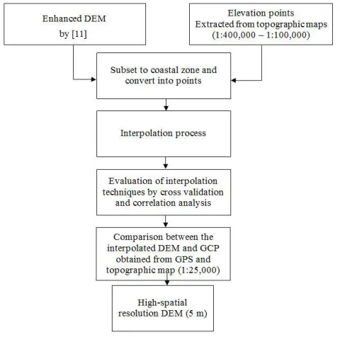
Next, elevations datasets were subset to correspond to the coastal zones of Kuwait and then converted to points. The elevation points were interpolated to refine the spatial resolution to 5 m. After that, the DEMs produced by different kinds of interpolation techniques were evaluated using a cross validation method and correlation coefficient
(r). The former method was performed by removing one elevation point and predicting this point with the model constructed using the remaining elevation points. The purpose of using cross validation was to evaluate the accuracy of the models in estimating unknown elevation values. For a best-fit model, the root mean square error (RMSE) should be as small as possible [12]. The latter method was used to calculate the association between the estimated elevation points and measured values of elevation points using correlation coefficient (r). Thereafter, the most acceptable interpolated DEM with lower RSME and higher (r) in each zone was selected. Then the interpolated DEM in each coastal zone were combined in one raster file. Then, the vertical accuracy of the interpolated DEM was examined by matching reference data (which were GCP obtained from both GPS and high-resolution topographic maps (1:25,000)), with corresponding elevation points in exact locations using linear regression coefficient (R2), following the procedure outlined by [11]. These GCP data were selected clear of buildings to fit spatially with data of the interpolated DEM. Figure 1 illustrates the flowchart of the methodology.
Figure 1. Methodology flowchart.
2.2. Study Area
Figure 2. The location of Kuwait and the coastal zones.
The coastal zone of Kuwait is a low-lying area, which makes it a prime location for the development of industries, residences, recreation, and tourism. The coast of Kuwait can be divided into three geographical regions: the north, which is non-urbanized; the south, including Kuwait Bay, which is heavily developed; and the south coast, which includes most of the industrial, commercial, and recreational areas. The topography of Kuwait is generally flat and decreases gradually from the southwest of the state toward the shoreline of the Arabian Gulf. The most prominent topographic area in the coastal zones of Kuwait is Jal Al-Zour. Its highest elevation reaches 145 m, and it is 60 km in length, north of Kuwait [13]. Kuwait’s coastal zones occupy an area of about 1,315 km2, extending nearly 10 to 20 km from the shoreline. Due to the different oceanographic characterizations in coastal region, and to facilitate the interpolation processes, this study divided the coastal zones of Kuwait into five zones: northern coast (zone 1), middle coast (zone 2), southern coast (zone 3), Boubyan Island (zone 4), and Failakah Island (zone 5).
2.3. Elevation Datasets
The DEM was utilized in this research for two reasons. First, it was spatially enhanced by [11]. Second, it is highly accurate in flat areas [14], which conforms to the topography of Kuwait’s coastal zone. GDEM, released in October 2011, has a spatial resolution, vertical accuracy, and horizontal accuracy of 30, 17, and 75 m, respectively. [11] matched elevation data retrieved from GDEM with 793 elevation points using regression analysis. They found that the relationship between elevations points and GDEM data was statistically significant and could be represented as the following:
Elevation = -0.0012GDEM2 + 1.2058 GDEM – 5.9763
By applying this model to GDEM data, the nominal vertical error was greatly reduced from 17 m to 5 m. They recommended using the enhanced DEM in the absence of highly accurate data, such as LiDAR data, because it is the best available source in terms of vertical accuracy. The first elevation data used in the interpolation process was obtained from the enhanced DEM after applying this model.
The second elevation data used in the interpolation process were obtained from topographic maps. [15] produced a contour map of Kuwait with a scale of 1:400,000 but without any spatial information; thus, the vertical and horizontal accuracies were calculated based on U.S. national map accuracy standards [16]. The vertical and horizontal accuracies for this map were 10 m and 203 m, respectively. The other topographic maps used were produced by the Defense Ministry of Kuwait, with scales of 1:100,000 and 1:25,000, using in situ data and aerial photography. Both of these maps have vertical and horizontal accuracies of 0.8 m and 5 m, respectively. However, elevation points from topographic maps with scales of 1:400,000 and 1:100,000 were used to conduct interpolation.
2.4. Interpolation Processes
Both deterministic and geostatistical interpolation techniques were used to generate the continuous surface of elevation data. The deterministic interpolation techniques included IDW and RBF, whereas the kriging method was applied as a geostatistical interpolation technique.
2.4.1. The Inverse Distance Weighting Method
Inverse Distance Weighting (IDW) method is a well-known interpolation technique that has been widely applied in different science fields. Inverse distance weighting predicts non-sampled locations using linearly weighted combinations of a set of sample points. This method was designed following [17] first law of geography, which states that near things are more related than distant things. Therefore, the closest points to the non-sampled location are weighted more greatly than distant points [18, 19]. The method is expressed as the following equation:
= ∑ ⁄ + ∑ 1 ℎℎ ⁄ (1)
where z(x0) is the interpolated value, n represents the total
number of sample data values, xi is the ith data value, hij is
the separation distance between the interpolated value and the sample data value, and ß denotes the weighting power.
2.4.2. The Radial Basis Function MethodRadial Basis Function (RBF) method covers a large series of exact, moderately quick interpolators (e.g., thin-plate spline (TPS), spline with tension (SPT), multiquadric function (MQ), completely regularized spline (CRS), and inverse multiquadratic function (IMQ)) that are used as a basic equation that is dependent on the distance between the predicted and the measured point [20]. Unlike the IDW method, the RBF predicts values above the maximum measured values and below the minimum measured values [21].
2.4.3. The Kriging Method
The kriging method is a sophisticated version of inverse distance interpolation that weights how much importance should be given to each neighbor location. There are several kinds of kriging, including simple kriging, ordinary kriging, and universal kriging. Ordinary kriging (OK) has been widely applied in interpolation processes due to its simplicity and prediction [22]. The weights of OK are derived from the kriging equations using a semivariance function. Semivariograms are commonly represented by plotting the difference squared between the values of each pair of locations on the y-axis relative to the distance separating each pair on the x-axis.
In this study, the following equation (2) was used to calculate the semivariogram:
ℎ = ( ) ∑ − + ℎ (2)
where z(xi) and z(xi+ h) are variable values on the xi, and xi+h
points, respectively, and N(h) is the number of paired sample points separated by distance h.
2.4.4. Accuracy Assessment
The interpolation methods applied to generate a high spatial resolution DEM were compared using cross validation. This was conducted by removing one data location and predicting the associated data using the data of the remaining locations. The accuracy of interpolation was done by calculating the deviations of interpolated elevation values from corresponding measured values in term of the Root Mean Square Error (RMSE):
= ∑ ∗ − (3)
where z(xi) is the observed value at location I, z*(xi) is the interpolated value at location i, and n is the sample size. Most researchers who have study DEMs and their applications proposed and used statistical measures, including the RMSE, to evaluate DEM reliability [23, 24]. Moreover, the correlation coefficient (r) was applied in order to examine the relationship between the predicted elevation points from the interpolated DEM and measured values taken from input spatial datasets. Higher values of (r) indicated higher significant correlations between datasets.
3. Results and Discussion
3.1. Determination Errors Using Cross Validation
The spatial resolution of the interpolated DEM was defined as 5 m rather than 30 m prior to the interpolation processes. The study area was divided into five major classes: northern coast (zone 1), middle coast (zone 2), southern coast (zone 3), Boubyan Island (zone 4) and Failakah Island (zone 5). Each zone was subjected to separate interpolation analysis. Table 1 represents the errors calculated using the cross validation method of the interpolation techniques in each zone. It is clear that the RBF interpolation technique obtains better results in all study zones (except for Failakah Island) compared to other interpolation techniques.
Table 1. Interpolation Methods and Corresponding Errors in Each Zone.
Interpolation method Model RMSE
Northern coast Middle coast Southern coast Boubyan Island Failakah Island
IDW 1.59 1.62 1.36 2.1 1.67
RBF Spline with tension 1.55 1.74 1.32 1.1 1.68
Interpolation method Model RMSE
Northern coast Middle coast Southern coast Boubyan Island Failakah Island
Multiquadric 1.57 1.56 1.33 1.08 1.69
inverse multiquadric 1.68 2.13 1.32 1.15 1.76
thin plate spline 1.57 1.34 1.11 1.82
Kriging
stable 1.68 1.69 1.68 1.15 1.74
circular 1.58 1.7 1.58 1.32 1.86
spherical 1.58 1.65 1.58 1.32 1.86
tetraspherical 1.58 1.57 1.54 1.32 1.86
pentaspherical 1.58 1.57 1.58 1.32 1.86
expnential 1.58 1.57 1.54 1.31 1.85
gaussian 1.68 1.74 1.68 1.33 1.87
rational quadratic 1.62 1.74 1.62 1.33 1.83
hole effect 1.68 1.74 1.68 1.33 1.87
k-Bessel 1.68 1.73 1.68 1.2 1.79
J-Bessel 1.68 1.74 1.68 1.33 1.87
In the northern coast (zone 1), the most suitable interpolation prediction with a low RMSE (1.55) was generated by the RBF (spline with tension). However, in the middle coast (zone 2), the RBF (multiquadric) achieved the best result with a low RMSE (1.56). In the southern coast (zone 3) and Boubyan Island (zone 4), the most suitable interpolated DEM was produced using the RBF (spline with tension) interpolation method, with an RMSE of 1.32 and 1.1, respectively. On the other hand, the IDW technique achieved the best result (RMSE = 1.67) compared to other interpolation methods used to generate DEMs in the Failakah Island area (zone 5).
Notably, using kriging as an interpolation technique did not demonstrate comparable results, and its estimations were mostly unrealistic. The deterministic interpolation methods reveal more accurate estimations for producing DEMs in the coastal zones of Kuwait than the geostatistical interpolation methods.
After combine the DEMs of each zone, the average error of the interpolation prediction was significantly decrease
(RMSE=1.44) comparing the original spatial data used to run the interpolation. [11] reduced the vertical error of GDEM by matching remotely sensed data with ground elevation points using regression analysis. The RMSE of their regression model was 5 m. Therefore, the RMSE data in the present study add to the RMSE of the above-mentioned study to obtain the overall error of the interpolated DEM, as shown in Table 2. The overall RMSE of the interpolated DEM was 6.44, indicating an increase of 28% compared to the original data (RMSE = 5).
Table 2. Overall RMSE of Interpolated DEM.
Study area Interpolation method RMSE Overall RMSE
Zone 1 RBF (spline with tension) 1.55 6.55
Zone 2 RBF (multiquadric) 1.56 6.56
Zone 3 RBF (spline with tension) 1.32 6.32
Zone 4 RBF (completely regularized) 1.1 6.1
Zone 5 RBF (spline with tension) 1.67 6.67
Average 1.44 6.44
3.2. Correlation Analysis
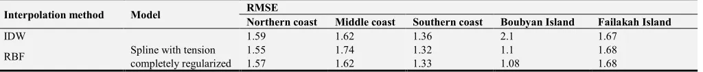
Figure 3. Scatter diagrams exhibit the association as correlation coefficients (r) between the predicted and measured elevation points in each zone. The
The degree of association between predicted and measured elevation points was examined using Pearson’s correlation coefficient (Figure 3). The correlation coefficients between tested data were significant, with p values below 0.01. The elevation data of both the predicted and measured values in the northern, middle, and southern coasts were highly correlated. Correlations between predicted and measured elevation points in both the Boubyan and Failakah Islands existed but were less associated.
3.3. Visual Enhancement of DEM
The visualization of DEM was substantially improved, as
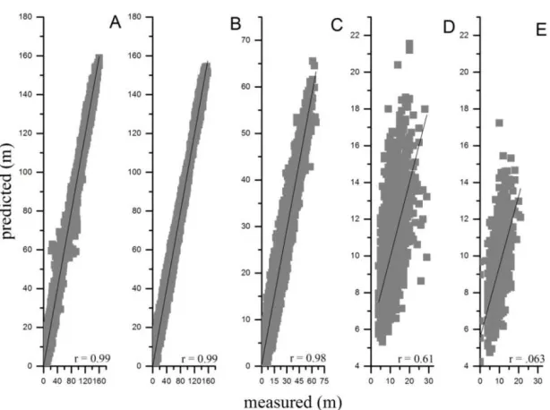
shown in Figure 4. The elevation profile (Figure 4A) in the original DEM had a spatial resolution of 30 m, which clearly shows lesser elevation bars, as in Figure 4C. In comparison, the interpolated DEM had a smaller pixel size, and the elevation bars were greater than the original DEM. The average pixel size of the original data was 30 m, but after the interpolation analysis, the pixel size was reduced to 5 m. The spatial resolution of the interpolated DEM was improved by 83% compared to the original data. The advantages of the spatial interpolation analysis amplify the effectiveness of the DEM on a local scale, in the absence of accurate elevation data.
Figure 4. Cross-section of elevations in the original data and the interpolated DEM. (A) the poor spatial resolution of the original data (30 m) was
represented by few elevation bars (C), while (B) shows the high spatial resolution of the interpolated DEM (5 m), as (D) displays more elevation bars.
3.4. Vertical Assessment of the Digital Elevation Model
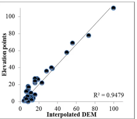
The reliability of the interpolated DEM was subjected to vertical assessment using GCP gathered from two different sources: GPS and a topographic map (1:25,000). The elevation points of these datasets were matched with the elevation data extracted from the interpolated DEM using linear regression coefficient (R2) at exact locations.
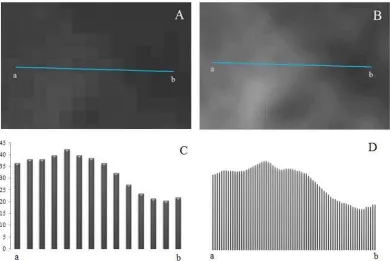
Elevation points from the interpolated DEM and GCP extracted from a topographic map (Figure 5) and in situ elevation data (Figure 6) were significantly correlated. In the first dataset, the elevation points from the topographic map were correlated with the interpolated DEM (R2 = 0.88), as shown in Figure 5. However, the correlation was higher between in situ elevation data and elevation data from the interpolated DEM (R2 = 0.94, Figure 6). These important correlations between both datasets make the interpolated DEM more reliable and effective to use in environmental fields in the coastal zone of Kuwait in absent of accurate
DEM.
Figure 5. The relationship between interpolated GDEM and elevation
Figure 6. The relationship between generated GDEM and elevation points obtained from field measurements.
4. Conclusions and Recommendations
The interpolation process provides variety of methods that enhance the spatial resolution of DEM. the interpolation methods were carried out on different spatial datasets including original DEM, counter maps, and elevation measurements that cover the five zones of Kuwait’s coastal area. The study shows that the interpolated DEM using deterministic methods such as RBF has RMSE lower than interpolated DEM using geostatistical methods. Moreover, the correlation coefficient (r) shows the significant association between predicted and measured elevation points with p values below 0.01 particularly in the zone 1, zone 2, and zone 3. The study demonstrates that elevation points from interpolated DEM matched significantly with elevation points extracted from high spatial resolution topography map and field measurements. The estimated error of interpolated DEM is about 1.44 m and that exceeds the error of spatial dataset employed in interpolation process but the spatial resolution of the interpolated DEM was enhanced significantly from 30 m to 5 m enabling further spatial analysis from national to local scale. With the lack of accurate DEM data, the interpolated DEM produced in this study may serve as a useful alternative to assess the geographic, geological and environmental issues that threaten the coastal area of Kuwait.
References
[1] Li, X., Shen, H., Feng, R., Li, J., & Zhang, L. DEM generation from contours and a low-resolution DEM. ISPRS Journal of Photogrammetry and Remote Sensing,2017, 134, 135–147.
[2] Pohjola, J., Turunen, J., & Lipping, T. Creating high-resolution digital elevation model using thin plate spline interpolation and Monte Carlo simulation. Working Report 2009-56. 2009, Pori, Finland: Tampere University of Technology.
[3] Yue, T.-X., Song, D.-J., Du, Z.-P., & Wang, W. High-accuracy surface modelling and its application to DEM generation.
International Journal of Remote Sensing,2010, 31 (8), 2205– 2226.
[4] Nelson, A., Reuter, H. I., & Gessler, P. DEM production methods and sources. Developments in Soil Science, 2009, 33, 65–85.
[5] Kobrick, M. On the Toes of Giants- How SRTM was Born.
Photogrammetric Engineering and Remote Sensing, 2006, 72 (3), 206–210.
[6] Carter, M., Shepherd, J. M., Burian, S., & Jeyachandran, I. Integration of lidar data into a coupled mesoscale–land surface model: A theoretical assessment of sensitivity of urban–coastal mesoscale circulations to urban canopy parameters. Journal of Atmospheric and Oceanic Technology,
2012, 29 (3): 328–346.
[7] Elkhrachy, I. Vertical accuracy assessment for SRTM and ASTER Digital Elevation Models: A case study of Najran city, Saudi Arabia. Ain Shams Engineering Journal. 2017. (article in press).
[8] Chaplot, V., Darboux, F., Bourennane, H., Leguédois, S., Silvera, N., & Phachomphon, K. Accuracy of interpolation techniques for the derivation of digital elevation models in relation to landform types and data density. Geomorphology,
2006, 77 (1-2), 126–141.
[9] Liu, L., Lin, Y., Liu, J., Wang, L., Wang, D., Shui, T., et al. Analysis of local-scale urban heat island characteristics using an integrated method of mobile measurement and GIS-based spatial interpolation. Building and Environment, 2017, 117, 191–207.
[10] ESRI. How IDW works. 2017a.
http://desktop.arcgis.com/en/arcmap/10.3/tools/3d-analyst-toolbox/how-idw-works.htm. Accessed 12 May 2017. [11] Alsahli, M. M. M., & Alhasem, A. M. Vulnerability of
Kuwait coast to sea level rise. Geografisk Tidsskrift-Danish Journal of Geography, 2016, 116 (1), 56–70.
[12] Nas, B., Karabork, H., Ekercin, S., & Berktay, A.. Assessing water quality in the Beysehir Lake (Turkey) by the application of GIS, geostatistics and remote sensing. In Proceedings of the 12th World Lake Conference, 2007, Taal (pp. 639–646). Jaipur, India.
[13] Al-Sarawi, M. A. Surface geomorphology of Kuwait.
GeoJournal, 1995, 35 (4), 493–503.
[14] Varga, M., & Bašić, T. Accuracy validation and comparison of global digital elevation models over Croatia. International journal of remote sensing, 2015, 36 (1), 170–189.
[15] Al-Sulaimi, J., & Mukhopadhyay, A. An overview of the surface and near-surface geology, geomorphology and natural resources of Kuwait. Earth-Science Reviews, 2000, 50 (3), 227–267.
[16] USGS. Routine ASTER global digital elevation model. 2016. https://lpdaac.usgs.gov/dataset_discovery/aster/aster_products _table/astgtm. Accessed 21 December 2017.
[18] Bhunia, G. S., Shit, P. K., & Maiti, R. Comparison of GIS-based interpolation methods for spatial distribution of soil organic carbon (SOC). Journal of the Saudi Society of Agricultural Sciences, 2016, 17 (2), 114–126
https://doi.org/10.1016/j.jssas.2016.02.001
[19] ESRI. Deterministic methods for spatial interpolation. 2017b. http://pro.arcgis.com/en/pro-app/help/analysis/geostatistical-analyst/deterministic-methods-for-spatial-interpolation.htm. Accessed 29 November 2017.
[20] Aguilar, F. J., Agüera, F., Aguilar, M. A., & Carvajal, F. Effects of terrain morphology, sampling density, and interpolation methods on grid DEM accuracy.
Photogrammetric Engineering & Remote Sensing, 2005, 71 (7), 805–816.
[21] Li, Y., Shi, Z., Wu, C.-F., Li, H. Y., & Li, F. Improved
prediction and reduction of sampling density for soil salinity by different geostatistical methods. Agricultural Sciences in China,2007, 6 (7), 832–841.
[22] Isaaks, E. H., & Srivastava, R. M. Applied geostatistics. (1989). New York: Oxford University Press.
[23] Cuartero, A., Polo, M. E., Rodriguez, P. G., Felicisimo, A. M., & Ruiz-Cuetos, J. C. The use of spherical statistics to analyze digital elevation models: An example from LiDAR and ASTER GDEM. IEEE Geoscience and Remote Sensing Letters, 2014, 11 (7), 1200–1204.