R E S E A R C H Open Access
Explicit maps to predict activation order in multiphase
rhythms of a coupled cell network
Jonathan E Rubin·David Terman
Received: 6 December 2011 / Accepted: 4 February 2012 / Published online: 12 March 2012 © 2012 Rubin, Terman; licensee Springer. This is an Open Access article distributed under the terms of the Creative Commons Attribution License (http://creativecommons.org/licenses/by/2.0), which permits unrestricted use, distribution, and reproduction in any medium, provided the original work is properly cited.
Abstract We present a novel extension of fast-slow analysis of clustered solutions to coupled networks of three cells, allowing for heterogeneity in the cells’ intrinsic dynamics. In the model on which we focus, each cell is described by a pair of first-order differential equations, which are based on recent reduced neuronal network models for respiratory rhythmogenesis. Within each pair of equations, one dependent variable evolves on a fast time scale and one on a slow scale. The cells are coupled with inhibitory synapses that turn on and off on the fast time scale. In this context, we analyze solutions in which cells take turns activating, allowing any activation order, including multiple activations of two of the cells between successive activations of the third. Our analysis proceeds via the derivation of a set of explicit maps between the pairs of slow variables corresponding to the non-active cells on each cycle. We show how these maps can be used to determine the order in which cells will activate for a given initial condition and how evaluation of these maps on a few key curves in their domains can be used to constrain the possible activation orders that will be observed in network solutions. Moreover, under a small set of additional simplifying assumptions, we collapse the collection of maps into a single 2D map that can be computed explicitly. From this unified map, we analytically obtain boundary curves between all regions of initial conditions producing different activation patterns.
Keywords fast-slow analysis·clustered solutions·map·multiphase rhythm· respiration
JE Rubin (
)Department of Mathematics, University of Pittsburgh, Pittsburgh, PA 15260, USA e-mail:[email protected]
D Terman
1 Introduction
The methods of fast-slow decomposition have been harnessed for the analysis of rhythmic activity patterns in many mathematical models of single excitable or os-cillatory elements featuring two or more time scales. In the analysis of relaxation oscillations, for example, singular solutions can be formed by concatenating slow trajectories associated with silent and active phases and fast jumps between these phases, and these can guide the study of true solutions. These methods can be pro-ductively extended to interacting pairs of elements, particularly when the coupling between them takes certain forms. The synaptic coupling that arises in many neu-ronal contexts is well suited for the use of this theory. In the case of synapses that turn on and off on the fast time scale, for example, analysis can be performed through the use of separate phase spaces for each neuron, with synaptic inputs modifying the nullsurfaces and other relevant structures in each phase space. This method has been used to treat pairs of neurons with slow synaptic dynamics as well, although higher-dimensional phase spaces arise. Similarly, synchronized and clustered solutions can be analyzed in model networks consisting of multiple identical neurons if these neu-rons are visualized as multiple particles in one phase space or in two phase spaces, one for active neurons and one for silent, the membership of which will change over time. Reviews of how fast-slow decompositions have been used to analyze neuronal networks can be found in, for example, [1,2].
This form of analysis becomes significantly more challenging when networks of three or more nonidentical neurons are considered. The number of variables in each slow subsystem can become prohibitive, and if variables associated with different neurons are considered in separate phase spaces, then some method is still needed for the efficient analysis of their interactions. In this study, we introduce such a method, based on mappings on slow variables, for networks in which each element is modeled with one fast variable and one slow variable, plus a coupling variable. A strength of this method is that, by numerically computing the locations of a few key curves in phase space, we can obtain information about model trajectories generated by arbi-trary initial conditions and determine how complex changes in stable firing patterns occur as parameters are varied. Moreover, the formulas defining approximations to these curves, valid under a small number of simplifying assumptions, can be ex-pressed in an elegant analytical form. These methods are particularly tractable within networks consisting of three reciprocally coupled units, so we focus on such networks here; also, we use intrinsic dynamics arising in neuronal models, although the theory would work identically for any qualitatively similar dynamics with two time scales.
we derive formulas for the times when each cell jumps up and down, and determine how these times depend on parameters and initial conditions. To derive these explicit formulas, we will make some simplifying assumptions on the equations; a similar analysis could be performed numerically if such explicit formulas could not be ob-tained. In Section4, we make some further simplifying assumptions that allow us to reduce the full dynamics to a piecewise continuous two-dimensional map. Analy-sis of this map helps to explain how complex transitions in stable firing patterns take place as parameters are varied. We conclude the article with a discussion in Section5.
2 Model system
2.1 Modeling respiratory rhythms
Recent work, based on experimental observations, has modeled the respiratory rhythm generating network in the brain stem as a collection of four or five neuronal populations. Three of these groups are inhibitory and are arranged in a ring, with each population inhibiting the other two. A fourth group, a relatively well-studied collection of neurons in the pre-Bötzinger Complex (pre-BötC), excites one of the inhibitory populations, also associated with the pre-BötC, and is inhibited by the other two. Finally, some studies have included a fifth, excitatory population, linked to certain other populations and likely becoming active only under certain strong per-turbations to environmental or metabolic conditions [4–8]. In addition to the synaptic inputs from other populations in the network, each neuronal group receives excita-tory synaptic drives from one or more additional sources, possibly related to feedback control of respiration (e.g., [9]). Under baseline conditions, the four core populations encompassed in this model generate a rhythmic output, in which the inhibitory groups take turns firing and the activity of the excitatory pre-BötC neurons slightly leads but largely overlaps that of the inhibitory pre-BötC cells.
The method that we present in this study has been developed to aid in the analyti-cal study of solutions of networks like the reduced respiratory population model. To make the presentation concrete, we present our results in terms of this model. Since two of the four active populations relevant to the normal respiratory rhythm, those in the pre-BötC, activate in near-synchrony, we will treat these as a single population and consider a three population network. The activity of one of the key respiratory brain stem populations depends on a persistent sodium current [10–13], while the other active populations feature an adaptation current instead [5,6]. In the three pop-ulation model that we use, we include this heterogeneity to illustrate that the theory handles heterogeneity easily, to distinguish one of the populations from the other two for ease of presentation of part of the theory, and to maintain a strong connection with the respiratory application.
2.2 The equations
The model equations we consider are
v1=F1(v1, h)−gI
b21S∞(v2)+b31S∞(v3)
(v1−VI)−gEd1(v1−VE), v2=F2(v2, m2)−gI
b12S∞(v1)+b32S∞(v3)
(v2−VI)−gEd2(v2−VE), v3=F3(v3, m3)−gI
b13S∞(v1)+b23S∞(v2)
(v3−VI)−gEd3(v3−VE), h=h∞(v1)−h
/τh(v1),
m2=m∞(v2)−m2
/τ2(v2), (1)
m3=m∞(v3)−m3
/τ3(v3).
Differentiation is with respect to timet, andis a small, positive parameter that we have introduced for notational convenience. In [6, 8], eachv variable denotes the average voltage over a synchronized neuronal population,h is the inactivation of a persistent sodium current for members of the inspiratory pre-BötC population, and themi represent the activation levels of an adaptation current for two other
respi-ratory populations; however, each variable could just as easily represent analogous quantities for a single neuron.
The functionsFiin (1) are given by:
F1(v1, h)= −
IN aP(v1, h)+IKdr(v1)+IL(v1)
/C,
F2(v2, m2)= −
Iad(v2, m2)+IL(v2)
/C, (2)
F3(v3, m3)= −
Iad(v3, m3)+IL(v3)
/C,
where C is membrane capacitance and IN aP(v, h) =gN aPmp∞(v)h(v −VN a), IKdr(v)=gKdrn∞4 (v)(v−VK),IL(v)=gL(v−VL), andIad(v, m)=gadm(v− VK) represent persistent sodium, potassium, leak and adaptation currents,
respec-tively. In each of these currents, the g parameter denotes conductance and the V
parameter is the current’s reversal potential. We use the standard convention of rep-resenting IN aP and IKdr activation as sigmoidal functions of voltage v,mp∞(v)
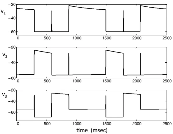
Fig. 1 A typical solution of system (1). There is always one and only one cell active at each time. When an active cell’s voltage reaches the synaptic thresholdθI, it jumps down releasing the other two cells from inhibition. There is then a race among these two cells to see which one crosses the synaptic threshold first. The winning cell becomes active and the other two cells return to the silent phase.
1//{1+exp[(v−θI)/σI]}, which closely approximates a Heaviside step function
due to the small size ofσI and which is multiplied by a strength factorbeach time
it appears. The final term,gEdi(vi−VE), in each voltage equation represents a tonic
synaptic drive from a feedback population; the strength factorsdi could change with
changing metabolic or environmental conditions, but we treat them as constants in this article. Additional details about the functions in (1) and (2), as well as parame-ter values used, are given in Appendix1. Appendix2also presents a general list of assumptions, satisfied by (1), (2) with the parameter values used, under which our theoretical methods will work.
3 Fast-slow analysis
3.1 Introduction
A typical solution of system (1) is shown in Figure1. Each of the cells lies in one of four states, which we denote as: (i) the silent phase; (ii) the active phase; (iii) the jump-up; and (iv) the jump-down. For example, in Figure1, att=0, cell 1 is active, while cells 2 and 3 are silent. At this time, cell 1 inhibits both of the other cells. This configuration is maintained untilv1(t )crosses the synaptic thresholdθI, at which
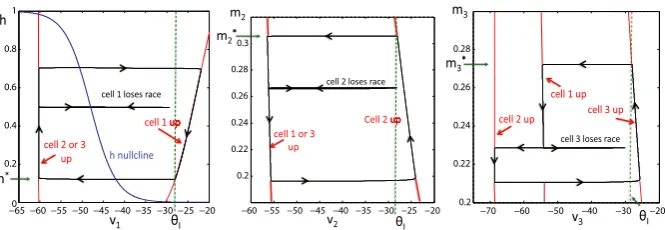
Fig. 2 The projections of the solution shown in Figure1onto the phase planes corresponding to the three cells. A cell lies on the left branch of itsv-nullcline while in the silent phase and on the right branch during the active phase. Jumps up and down between these branches are initiated when an active cell reaches the synaptic thresholdθI, which occurs ath=h∗,m2=m∗2, orm3=m∗3, respectively.
discussed shortly). There is then a race to see which of the voltages,v2(t )orv3(t ), crosses the thresholdθI first. Suppose thatv2crossesθI first, as in the first transition
that occurs in Figure1. When this happens, cell 2 sends inhibition to both cells 1 and 3, so both of these cells must return to the silent phase. Hence, cell 2 is now active, while the other two cells are silent. These roles persist untilv2(t )crosses the synaptic thresholdθIand releases cells 1 and 3 from inhibition, at which time there is another
race to see whether cell 1 or cell 3 crosses threshold first. This process continues, with one of the cells always lying in the active phase until its membrane potential crosses threshold and releases the other two cells from inhibition. The projections of this solution onto the phase planes corresponding to the three cells are shown in Figure2.
We analyze solutions using fast-slow analysis. The basic idea is that the solu-tion evolves on two different time scales: During the jumps up and down, the so-lution evolves on a fast time scale, while during the silent and active phases, the solution evolves on a slow time scale. The fast-slow analysis allows us to derive re-duced equations that determine the evolution of the solution during each of these phases. In particular, we derive explicit formulas for the times when each cell jumps up and down and use these to determine the outcomes of the races to threshold, de-pending on parameters and initial conditions. To derive these formulas, we will make some simplifying assumptions on the equations; in situations in which such formulas cannot be obtained, then a similar analysis can be done numerically.
3.2 Slow and fast equations
We first consider equations for the slow variablesh,m1andm2. These equations are obtained by introducing the slow time scale,τ =t, and then setting =0 in the resulting equations. These steps give:
0=F1(v1, h)−gI
b21S∞(v2)+b31S∞(v3)
(v1−VI)−gEd1(v1−VE),
0=F2(v2, m2)−gI
b12S∞(v1)+b32S∞(v3)
(v2−VI)−gEd2(v2−VE),
0=F3(v3, m3)−gI
b13S∞(v1)+b23S∞(v2)
h=h∞(v1)−h
/τh(v1),
m2=m∞(v2)−m2
/τ2(v2), (3)
m3=m∞(v3)−m3
/τ3(v3),
where differentiation is with respect toτ. To simplify the analysis, we take the ex-treme (v→ ±∞) values of each of the functionsh∞,m∞,τh,τ2, andτ3and replace each function with a step function that jumps abruptly between these values. That is, we assume that there are positive constantsσL,σR,λL,λR,μLandμR(see Tables1
and2 in Appendix1, singular limit parameter values) such that the slow variables satisfy equations of the form:
h(t )=
σL(1−h) if cell 1 is silent, −σRh if cell 1 is active,
m2(t )=
−λLm2 if cell 2 is silent,
λR(1−m2) if cell 2 is active,
m3(t )=
−μLm3 if cell 3 is silent,
μR(1−m3) if cell 3 is active. We solve these equations explicitly to obtain:
h(τ )=
1+h(0)−1e−σLτ if cell 1 is silent,
h(0)e−σRτ if cell 1 is active, (4)
m2(τ )=
m2(0)e−λLτ if cell 2 is silent, 1+m2(0)−1
e−λRτ if cell 2 is active, (5)
m3(τ )=
m3(0)e−μLτ if cell 3 is silent, 1+m3(0)−1
e−μRτ if cell 3 is active. (6)
We next consider the fast time scale, which is simplyt. Let=0 in (1) to obtain the fast equations:
v1 =F1(v1, h)−gI
b21S∞(v2)+b31S∞(v3)
(v1−VI)−gEd1(v1−VE), v2 =F2(v2, m2)−gI
b12S∞(v1)+b32S∞(v3)
(v2−VI)−gEd2(v2−VE), v3 =F3(v3, m3)−gI
b13S∞(v1)+b23S∞(v2)
(v3−VI)−gEd3(v3−VE),
h=m2=m3=0. (7)
Note that the slow variables are constant on the fast time scale. We will only explicitly solve the fast equations when there is no inhibition; that is, we will solve these equa-tions to determine what happens when the cells are released from inhibition (which we take to be att=0) and jump up, competing to become active next. In this case, eachS∞=0. We note that the fast equations forv2andv3are both linear and can be solved explicitly. If there is no inhibitory input then, fork=2 or 3,
vk(t )=Ak+
vk(0)−Ak
SinceVE=0 (see Tables1and2in Appendix1), this gives
Ak=
gadmkVK+gLVL gadmk+gL+gEdk
and Bk=gadmk+gL+gEdk.
To obtain an explicit formula forv1(t ), we will make some simplifying assumptions. First, since the voltage values for cell 1 during the silent phase and most of the jump up lie in a range where the potassium activation functionn∞(v)is quite small, we assume thatn∞(v1)is negligible throughout these phases. Moreover, we assume that the sodium gating variablemp∞(v)is a step function. That is, there is a threshold
value,Vmp< θI, so thatmp∞(v)=0 ifv < Vmpandmp∞(v)=1 ifv > Vmp. In this
case, the fast equation forv1is piecewise linear, and we can write its solution as
v1(t )=
A1+
v1(0)−A1
e−B1t, 0≤t < t mp, ˆ
A1+(Vmp− ˆA1)e− ˆB1(t−tmp), tmp≤t,
(9)
where
A1=gLVL/B1, B1=gL+gEd1,
ˆ
A1=(gN aPhVN a+gLVL)/Bˆ1, and Bˆ1=gN aPh+gL+gEd1, with
tmp=
1
B1
lnB1v1(0)−gLVL
B1Vmp−gLVL .
3.3 The race
As described above, when one of the cells jumps down, there is a race to see which of the other cells reaches threshold first and then inhibits the other cells. Here we derive formulas that determine which cell wins the race to threshold.
First suppose that cell 1 jumps down from the active phase and releases cells 2 and 3 from inhibition. We need to determine the times it takes for the membrane potentials of these two cells to reach the synaptic threshold. While jumping up, these membrane potentials satisfy (8), so once we determine the initial conditionsvk(0), k=2,3, we can solve for the jump-up times.
While cells 2 and 3 are in the silent phase, they lie on the slow nullclines given by the second and third equations in (3) withS∞(v1)=1 andS∞(v2)=S∞(v3)=0. Given any values ofm2andm3, we can solve these equations explicitly forv2andv3 to conclude that at the moment that cells 2 and 3 begin to jump up,
vk(0)=
gadmkVK+gLVL+gIb1kVI gadmk+gL+gIb1k+gEdk ≡
Vk1, (10)
wherek=2 or 3. Substituting this expression into (8) and settingvk(tk1)=θI, we
find that the jump-up times are given by
tk1(mk)=
1
Ck1 ln
Dk1
Ek1
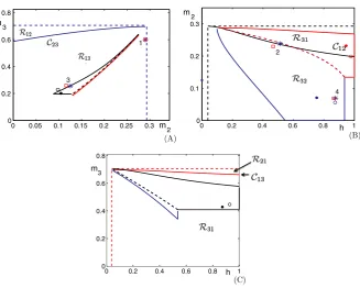
Fig. 3 Jumping regions in the slow phase planes.(A)(m2, m3)plane.(B)(h, m2)plane.(C)(h, m3) plane. Curves and color codes are described in detail in the text.
where
Ck1=gadmk+gL+gEdk,
Dk1=gadmk(Vk1−VK)+gL(Vk1−VL)+dkgEVk1 and
Ek1=gadmk(θI−VK)+gL(θI−VL)+dkgEθI.
Now, either cell 2 or cell 3 will win the race, if either t21(m2) < t31(m3) or
t21(m2) > t31(m3), respectively. The equationt21(m2)=t31(m3)defines a curve in the(m2, m3)plane, which we denote asC23. An example of this curve is shown in Figure3A, where we numerically solved forC23for parameter values given in Table1 in the Appendix. Points above this curve correspond to cell 2 winning the race and points below this curve correspond to cell 3 winning the race.
n∞(v1)=0. These steps give
vj(0)=
gadmjVK+gLVL+gIbkjVI gadmj+gL+gIbkj+gEdj
≡Vj k, (12)
v1(0)=
gLVL+gIbk1VI gL+gIbk1+gEd1≡
V1k. (13)
As with the derivation of (11), substitutingvj(0)into (8) yields
tj k(mj)=
1
Cj k
ln
Dj k Ej k
, (14)
where
Cj k=gadmj+gL+gEdj,
Dj k=gadmj(Vj k−VK)+gL(Vj k−VL)+djgEVj k
and
Ej k=gadmj(θI−VK)+gL(θI−VL)+djgEθI.
To compute t1k(h), we plug V1k into (9) and solve for v1(τ ) =θI. Recall that mp∞(v)=0 ifv < Vmp andmp∞(v)=1 ifv > Vmp, as reflected in the piecewise
formulation of (9). Thus, this calculation yields two terms, one corresponding to the time beforevreachesVmpand one to the time after, namely
t1k(h)=
1
C1ka
ln
D1ka E1ka
+ 1 C1kb
ln
D1kb E1kb
, (15)
where
C1ka=gL+gEd1,
D1ka=gL(V1k−VL)+gEd1V1k, E1ka=gL(Vmp−VL)+gEd1Vmp, C1kb=gN aph+gL+gEd1,
D1kb=gN aph(Vmp−VN a)+gL(Vmp−VL)+gEd1Vmp, E1kb=gN aph(θI−VN a)+gL(θI−VL)+gEd1θI.
Now, cell 1 will either win or lose the race, if eithert1k(h) < tj k(mj)ort1k(h) > tj k(mj), respectively. Each equationt1k(h)=tj k(mj)defines a curve in the(h, mj)
plane, which we denote asC1j. These curves are also shown in Figure3, where we
numerically solved forC12andC13. Note that points above the curveC1jcorrespond
3.4 Predicting jumping sequences
We now construct six 2D maps,ij, that allow us to predict the order in which the
cells jump up and down, to and from the active phase. To explain what these maps are, suppose thati,j andkare the cells’ distinct indices and, for convenience, tem-porarily lets1=h,s2=m2,s3=m3 denote the slow variables for the three cells. If, at some time, cellijumps down and cellkjumps up, then we will define a map
ik from the(sj, sk)phase plane to the(si, sj)phase plane that gives the position of (si, sj)when cellkjumps down. We can determine the next cell to jump up, once cell kjumps down, by comparing the position ofik(sj, sk)to that ofCij. For example,
suppose that cell 1 jumps down. Then either cell 2 or cell 3 will jump up depend-ing on whether(m2, m3)lies above or below the curveC23, respectively. If cell 2 jumps up, then the map12(m2, m3)gives the position of(h, m3)when cell 2 jumps down. This position, in turn, determines whether cell 1 or cell 3 is the next cell to jump up; that is, cell 1 or cell 3 is the next cell to jump up if(h, m3)=12(m2, m3) lies above or belowC13, respectively. Continuing in this way - comparing the out-put of the maps to the location of curvesCij - we can determine the cells’ jumping
sequences.
We derive explicit formulas for the six mapsij. The first step is to determine
the value of the slow variable for cell i when cell i jumps down. We claim that there exist unique constantssi∗so that cellijumps down whensi=si∗; see Figure2,
wheres1∗=h∗,s2∗=m∗2ands3∗=m∗3. These constants exist and are unique because: (i) celli jumps down when it is in the active phase withvi =θI; (ii) while celliis
in the active phase,(vi, si)lies along the right branch of thevi-nullcline,{(vi, si): Fi(vi, si)−gEdi(vi−VE)=0}; and (iii) each of these right branches is monotone
increasing or decreasing. This last statement can be verified for the concrete model (1) given in Section2by explicitly solving for eachsi in terms ofvi. However, this
monotonicity is also present in most reduced models for neuronal activity.
We now resume usingh,m2,m3to denote the slow variables for the three cells. First suppose that cell 1 is active; it will jump down whenh=h∗. Let us say that this occurs at timeτ =0, withmj=mj(0)forj=2,3, and that cellk,k=2 or 3,
wins the race and jumps up next; note that sinceτ is the slow time,τ =0 continues to hold throughout the jump. While cellkis up,hwill increase, mk will increase,
andmj,j=k, will decrease, governed by Equation (3). This state will persist until mk reachesm∗k. From the active component of Equation (5) or (6), we can solve mk(τ )=m∗kto compute the slow timeTkAfor which cellkremains active,
TkA= 1 νR
ln
1−mk(0)
1−m∗k
,
whereνR∈ {λR, μR}as appropriate. While cellk is active,his given by the silent
part of Equation (4) with h(0)=h∗ andmj,j =k, is given by the silent part of
Equation (5) or (6). From these equations, we can evaluateh(TkA),mj(TkA), and we
define the map1kby 1k
mj(0), mk(0)
=hTkA, mj
Specifically,
12
m2(0), m3(0)
=hT2A, m3
T2A
=1+h∗−1 σL/λR2 , m3(0) 2μL/λR
(16)
and
13
m2(0), m3(0)
=hT3A, m2
T3A =1+h∗−1 σL/μR
3 , m2(0)
λL/μR
3 , (17) where j=
1−m∗j/1−mj(0)
(18)
forj∈ {2,3}.
If the output of1k in the(h, mj)plane is above or below the curveC1j, then
cell 1 or cellj jumps up after cellk, respectively. Similarly, if we apply1k to the
entire region in the positive(j, k)quadrant lying below curveCj k, corresponding to
cellkjumping after cell 1, then we can determine which, if any, initial(mj, mk)cause
cellj to jump after cellkand which, if any, lead to cell 1 jumping after cellk. Note that for analyzing possible repetitive solutions, we really only need to consider inputs to1k that satisfy
0≤m2≤m∗2, 0≤m3≤m∗3. (19) This constraint is appropriate because if, for example,m2> m∗2, then once cell 2 is released from inhibition and jumps up, it can never reach the thresholdv2=θI.
Using a similar approach, based on computing an active time from the active com-ponent of one of the Equations (4), (5), and (6) and tracking the evolution of the slow variables of the two silent cells with the silent parts of the remaining two equa-tions from this set, the mapsij can be defined for each combination ofi=j from {1,2,3}. The mapijtakes values of the slow variables of cellsj andk,i=j=k, as
inputs, and gives values of the slow variables of cellsiandkas outputs. In particular, for each pairj, k∈ {2,3}withj=k, we have
j k
h(0), mk(0)
=hTkA, mj
TkA
=1+h(0)−1 kσL/νR, m∗j ωL/νRk (20)
and
j1
h(0), mk(0)
=mj
T1A, mk
T1A =
m∗j
h∗ h(0)
ωL/σR , mk(0)
h∗ h(0)
νL/σR
, (21)
where kis defined in (18) and where(ν, ω)=(λ, μ)ifk=2 while(ν, ω)=(μ, λ)
for repeated states, using (19) and
h∗≤h≤1. (22)
If celli jumps down at time 0 and the inputs to the map specify that cellj jumps next, then the location of the coordinate determined by the outputs ofij, relative
to the curveCik, determines whether cellior cellkwill follow cellj into the active
phase.
Taken collectively, the curves and maps defined in this section gives us a complete view of the possible jump sequences that system (1) can generate, at least if is small enough to justify the fast-slow decomposition that we have used. Consider the regions in the(m2, m3),(h, m2), and(h, m3)phase planes that satisfy (19) and (22). Within the(m2, m3)plane, assume that the curve C23 intersects the relevant region; otherwise, cell 1 will always be followed by the same other cell. The map
12 takes the region above the curve to a set in the(h, m3)plane and the map13 takes the region below the curve to a set in the(h, m2)plane, with similar actions for 21, 23, 31,32 on the other planes. Since the solutions to the ODEs we consider are continuous in initial conditions, the maps take connected regions into connected regions, and thus we only need to consider the actions of the maps on the regions’ boundaries in order to determine the possible next outcomes from a given starting point. For a particular parameter set, repeated iteration of the maps may show convergence to a single attracting jump sequence or may otherwise constrain the jump orders that are possible. Alternatively, inverses of the maps can be easily defined using the backwards flow of the ODEs, and repeated iterations of the inverses of the maps, applied to some selected region in one of the phase planes, show which sets contain initial conditions that could end up in the selected region.
3.5 Numerical examples
We now use numerical computations, performed with MATLAB and XPPAUT (http://www.pitt.edu/~phase), to illustrate the theory from the previous subsections. Figure3shows curves and regions in each of the 2D phase planes associated with pairs of slow variables of model (1). These structures were generated by starting from the full model, with function and parameter values given in the Appendix (see Table1), and making the simplifying assumptions described above for the=0 limit (including adjustingθmto−54 mV from−50 mV to compensate for the switch from
a smooth function to a Heaviside in the singular limit). In each panel, the relevant region can be defined using (19), (22), and the dashed straight line segments are boundaries of this region, each corresponding toh∗,m∗2, orm∗3. Within each region, there is a curveCij that separates initial conditions that lead to different jumping
Similar regions are indicated in black in the(h, m2)plane in Figure3B and in red in the(h, m3)plane in Figure3C.
Consider again the(m2, m3)plane shown in Figure3A. The regionR12is mapped by12to a connected region in the(h, m3)plane. In Figure3C, we represent part of the boundary of12(R12):= {12(m2, m3):(m2, m3)∈R12}with blue curves, car-rying over the coloring ofR12from Figure3A. Similarly, a regionR32belowC12in the(h, m2)plane in Figure3B also yields jumping by cell 2 and is mapped by32to a connected region in the(h, m3)plane. We indicate this region with black boundary curves in Figure3C, carrying over the coloring from Figure3B. The regions outlined in black and blue in the(h, m3)plane share a common boundary, corresponding to the condition that(h, m3)=(h∗, m∗3)when cell 2 jumps up. We use a dashed black line to denote this common boundary in Figure3C (by arbitrary convention, we color the dashed line to match the upper set). Now, the entire regions outlined in blue and black in the(h, m3)plane lie below the red curveC13 (Figure3C). Thus, we imme-diately know that, no matter what happened before, cell 3 will win the race and jump up when cell 2 jumps down. Similarly, in the(m2, m3)plane shown in Figure3A, the black-bounded region31(R31)and the red-bounded region21(R21)lie entirely belowC23, and therefore cell 3 will always jump up after cell 1 as well.
The interesting case in this example arises in the(h, m2)plane. There,13(R13), outlined in solid blue and dashed red, and23(R23), outlined in solid and dashed red, are both intersected byC12. Hence, there are initial conditions in our relevant regions for which the jump sequence 1,3,1 occurs and others for which the jump sequence 1,3,2 occurs, and similarly, there are initial conditions leading to jump sequences 2,3,1 and 2,3,2 as well. We can now summarize all possible jump sequences for the parameter set used in this example:
1→←3→←2,
possibly discarding a brief transient.
We also performed direct numerical simulations of system (1), using steep but smooth sigmoidal functions instead of Heaviside functions form∞(v),n∞(v), and
S∞(v), as described in the Appendix. These simulations also gave a 13231323. . . fir-ing pattern, as predicted by the analysis. We defined firfir-ing transitions in these simu-lations using voltage decreases through−33 mV (the half-activation of the synaptic functionS∞(v) was set to−32 mV to agree with θI). We allowed the system to
converge to its stable firing pattern and then plotted the slow variable coordinates at these firing transitions as open circles in the corresponding panels of Figure3. These coordinates agree well with the singular limit analysis.
In addition to the solid and open circles corresponding to the attractors in the sin-gular limit and full simulations, respectively, certain points associated with transients are also plotted in Figure3. An example of a transient 1,3,1,3 firing sequence found with the singular limit formulas, which led to a subsequent 2313231323. . . activation pattern, is marked with the blue asterisks in Figure3A,B. In this example, initial conditions were chosen such that cell 1 jumped down with(m2, m3)=(0.29,0.6), indicated by the rightmost asterisk in Figure3A (label 1). Since the asterisk is below the blue solid curveC23 in the plane shown, cell 3 jumps next. Obviously, the im-age of the initial point under13 must lie in the range of13 in the(h, m2)plane, which is bounded to the left, below and to the right by solid blue curves and above by a dashed red curve. We observe (Figure3B, label 2) that this image lies at about
(h, m2)=(0.51,0.24), which is indeed in the relevant region but also is above the black solid curveC12, meaning that cell 1 jumps up next. The image of(h, m2)under
31is marked by the other asterisk in Figure3A (label 3), which lies belowC23such that cell 3 jumps again after cell 1. Finally, the image of that point under13 is la-beled by the other asterisk in Figure3B (label 4); since that point is below the black curveC12, cell 2 finally gets to fire after this second activation of cell 3.
We also obtained a similar 1,3,1,3 transient in full model simulations correspond-ing to the scorrespond-ingular limit analysis. To match the scorrespond-ingular limit, we used(m2, m3)=
(0.29,0.6)as our initial condition, withv1= −33 mV andh=h∗such that time 0 represented the beginning of the jump down of cell 1. This point and the slow vari-able values at the next 3 jump down transitions are marked with red open squares in Figure3. By construction, the red open square at label 1 lies in the same position as the blue asterisk there. The rest of these markers, near labels 2,3,4, lie quite close to the blue asterisks, showing that, in addition to correctly predicting the jumping se-quence, the singular limit analysis gives good estimates to the slow variable values at jumping times in the original system, although the agreement is not perfect since
is nonzero in the original system and our analysis replaces sigmoidal activation and coupling functions by step functions.
4 From six maps to one
4.1 Derivation of the map
and(m2, m3). Here, we demonstrate that it is possible to use these six maps to reduce the dynamics to a single map, defined from some subset of the(m2, m3)phase plane into itself. Moreover, with some simplifying assumptions, we will derive an explicit formula for the map.
First, fix(m2, m3)and assume that whenτ=0, cells 2 and 3 lie in the silent phase withm2(0)=m2andm3(0)=m3. Suppose also that cell 1 lies in the active phase withv1(0)=θI, so that cell 1 jumps down at this time. Then either cell 2 or cell 3
will jump up. These two cells may take turns firing, but we assume that eventually, cell 1 will win a race and successfully jump up to the active phase again, from which it will subsequently jump down and start a new cycle. ChooseT >0 to be the first time (afterτ =0) that cell 1 jumps down. Then define a map as simply
(m2, m3)=
m2(T ), m3(T )
. (23)
In other words, iterates ofkeep track of the positions of(m2, m3)every time that cell 1 jumps down from the active phase.
We can obtain explicit formulas for this map if we assume that the slow variables satisfy (4), (5), and (6). Different sets of formulas will be relevant on the regionsR12 orR13, above or belowC23 respectively, corresponding to whether cell 2 or cell 3 wins the race and jumps up first when cell 1 jumps down. We can subdivide each of these regions based on the number of times that cells 2 and 3 take turns firing after cell 1 jumps down, before cell 1 jumps up again. On each of these subregions of the(m2, m3)phase plane, a different formula applies. Here we derive the formulas for the case in which cell 2 jumps up atτ =0 when cell 1 jumps down. Formulas for the case in which cell 3 jumps up atτ =0 are derived in a similar manner. First we derive the formulas for the map and then determine for which region of the
(m2, m3)phase plane each component of the formula is valid.
Recall that cells 2 and 3 may take turns firing for 0≤τ < T. LetN2andN3be the number of times that cells 2 and 3, respectively, jump up during this time interval. We note that either the two cells fire the same number of times, in which caseN3=N2, or cell 2 fires one more time than cell 3, in which case N3=N2−1. Using the definitions and notation described in the preceding section, we find that:
IfN3=N2, then
(m2, m3)=31◦23◦(32◦23)N2−1◦12(m2, m3). IfN3=N2−1, then
(m2, m3)=21◦(32◦23)N2−1◦12(m2, m3).
We derive explicit formulas for these maps using the formulas forij derived in the
preceding section. In what follows, we use the notation(m2, m3)=(mˆ2,mˆ3), and we employ the time constantsσL,σR,λL,λR,μLandμRintroduced in Section3.2.
Case 1:N2=1,N3=0.
Here(mˆ2,mˆ3)=21◦12(m2, m3)=21(h1, m13), where
h1=1+h∗−11−m
∗
2 1−m2
σL/λR
, m13=m3
1−m∗2
1−m2
μL/λR ,
ˆ m2=m∗2
h∗ h1
λL/μR
, mˆ3=m13
h∗ h1
μL/λR .
(24)
To achieveN3=0, we need that cell 1, not cell 3, jumps up when cell 2 jumps down. From the earlier discussion, this is true if(h1, m13)lies above the curveC13. Together with (24), this criterion leads to a condition on(m2, m3), which defines a region in the
(m2, m3)plane where this case occurs. One could numerically compute this region using the definition ofC13 given in the preceding section. Alternatively, we will now make a simplifying assumption that allows us to compute this region analytically. The validity of this assumption will be confirmed by comparing the firing sequence of the full model with that predicted by the analysis in the examples in the following section.
Our simplifying assumption can be described as follows: Suppose that at some time, sayt =0, cell 1 lies in the silent phase and is released from inhibition (by either cell 2 or cell 3). We assume that the time it takes cell 1 to jump up and reach the thresholdθI is independent ofh(0). It follows from this assumption that the curves C12andC13are horizontal; that is, they can be written asm2=M2andm3=M3for some constantsM2andM3.
Using this assumption, we conclude that Case 1 occurs if: (a)(m2, m3)lies above
C23 (so that cell 2 jumps up when cell 1 jumps down), and (b) m13> M3, which, together with (24), gives
m3> M3
1−m2 1−m∗2
μL/λR
≡k21(m2). (25)
We define the curveK12by
K2 1:=
(m2, m3)∈R12:m3=k12(m2)
.
Here, the superscript ‘2’ reflects that cell 2 jumps up when cell 1 jumps down, while the subscript ‘1’ corresponds to the number of jumps that follow before cell 1 jumps up again (i.e.,N2+N3=1). There is another curve, given bym2=K31(m3), corre-sponding to cell 3 jumping up when cell 1 jumps down. The formula forK31is derived in a similar manner, andK31⊂R13, belowC23.
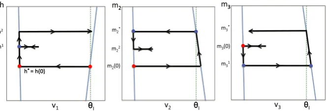
Case 2:N2=1,N3=1.
This case is illustrated in Figure4. Here,
(mˆ2,mˆ3)=31◦23◦12(m2, m3)=31◦23
h1, m13=31
Fig. 4 Phase planes for Case 2. We start at the red disc, when cell 1 jumps down from the active phase (or equivalently, with respect to the slow timeτ, when cell 1 enters the silent phase). At this time, cell 2 wins the race and jumps up. When cell 2 jumps down, cell 3 wins the race with cell 1 and jumps up. Finally, when cell 3 jumps up, cell 1 wins the race with cell 2 and jumps up.
where
h2=1+h1−11−m
∗
3 1−m13
σL/μR
, m22=m∗2
1−m∗3
1−m13
λL/μR ,
ˆ m2=m22
h∗ h2
λL/σR
, mˆ3=m∗3
h∗ h2
μL/σR ,
(26)
whereh1,m13are defined in (24). For this case to occur, we need that: (i) cell 3 jumps up when cell 2 jumps down, and (ii) cell 1 jumps up when cell 3 jumps down. These conditions are satisfied if: (i)(h1, m13)lies below the curveC13, and (ii)(h2, m22)lies above the curveC12. These conditions define a region in the(m2, m3)phase plane. If we make the same assumption as in Case 1, that the curvesC12andC13 are given bym2=M2andm3=M3 for some constantsM2andM3, then Case 2 occurs if: (a)(m2, m3)lies aboveC23(i.e., inR12), (b)m13< M3, and (c)m22> M2. It follows from (24) and (26) that (b) and (c) are satisfied ifk22(m2) < m3< k21(m2)where
k22(m2):=
1−(m∗2 M2)
μR/λL(1−m∗
3)
(1−m∗2)μL/λR (1−m2)
μL/λR. (27)
Furthermore, we define the boundary curve
K2 2=
(m2, m3)∈R12:m3=k22(m2)
,
such that Case 2 corresponds to those(m2, m3)∈R12betweenK12andK22.
General case: The general formulas are derived recursively, again by direct calcu-lation. Let
α=m∗21−m3∗λL/μR, β=m∗
3
1−m∗2μL/λR, f (m)=α(1−m)−λL/μR, g(m)=β(1−m)−μL/λR,
mk3=(g◦f )k−1m13 ifkis odd,
ak=
⎧ ⎪ ⎪ ⎪ ⎨ ⎪ ⎪ ⎪ ⎩
1−m∗2
1−mk−2 2
σL/λR
ifkis oddhere, we letm−21=m2
,
1−m∗3
1−mk3−2
σL/μR
ifkis even,
h0=1+h∗−1a1, (28)
hk=ak+1hk−1+1−ak+1 fork≥1, (29)
andN=N2+N3. Then(m2, m3)=(mˆ2,mˆ3), where
ˆ m2=
⎧ ⎪ ⎪ ⎨ ⎪ ⎪ ⎩
m∗2
h∗ hN
λL/σR
ifN2=N3,
mN2
h∗ hN
λL/σR
ifN2=N3,
(30)
and
ˆ m3=
⎧ ⎪ ⎪ ⎨ ⎪ ⎪ ⎩
mN3
h∗ hN
μL/σR
ifN2=N3,
m∗3
h∗ hN
μL/σR
ifN2=N3.
(31)
Formulas (30) and (31) hold only if cells 2 and 3 take turns firingN2andN3times, respectively, before cell 1 finally jumps up. As before, we can use the explicit formu-las forhk,mk2,mk3to derive explicit conditions on the initial point(m2, m3)for when this is true. We do not give the explicit general formula here. In the following section, we consider concrete examples and will give the formulas needed for the analysis of those examples.
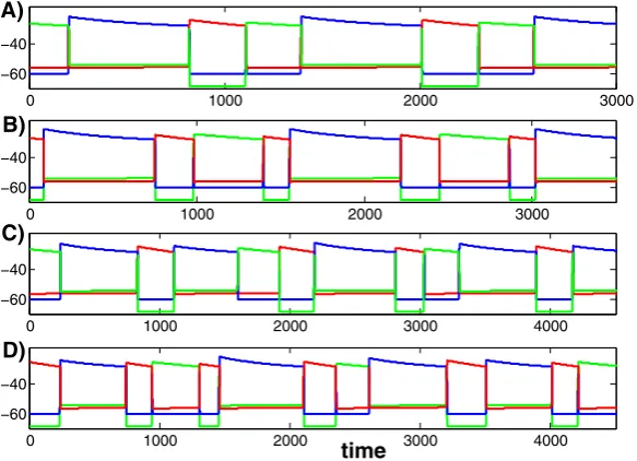
4.2 Numerical examples
Again, we use MATLAB and XPPAUT to illustrate our results numerically. Figure5 shows four solutions of system (1), each generating a different firing pattern, corre-sponding to parameter values given in the Appendix in Table2. The parameters for each of these solutions are exactly the same except for the ratesλLandμLat which
the slow variablesm2andm3decay while cells 2 and 3 lie in the silent phase. Here we show stable attractors so the firing patterns presented repeat as time evolves. In each panel, cells 1, 2, and 3 are displayed with the colors blue, green and red, re-spectively. We can denote the firing patterns shown in Figure5A-D as (132), (1323), (13123132), and (132313213), respectively, in reference to the shortest firing pattern that repeats in each case. The analysis presented in Section4.1is very useful in un-derstanding the origins of these firing patterns and how transitions between the firing patterns take place as parameters are varied.
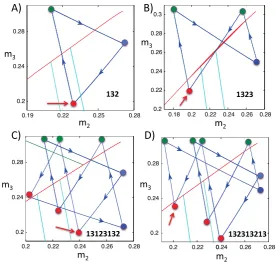
Figure 6 shows the projections of the solutions exhibited in Figure 5 onto the
Fig. 5 Four solutions of (1) for different values of the parameters(λL, μL), given in the text. In each panel, theblue,greenandred curvescorrespond to cells 1, 2, and 3, respectively.
the solution shown in Figure5A onto the(m2, m3)phase plane. For this solution,
(λL, μL)=(1/3,500,1/2,000). The red, blue, and green circles correspond to when
cells 1, 2, and 3 jump down, respectively. The red curve corresponds toC23 and the two turquoise curves correspond toK31(to the right of/above the red circle) andK32 (to the left of/below the red circle), respectively. If we start at the red circle (at the arrow) and follow the blue trajectory, then we find that cells 1, 3, and 2 take turns firing, in that order. Note that when cell 1 jumps down,(m2, m3)lies belowC23, such that cell 3 jumps after cell 1, andk23(m3) < m2< k31(m3). This position corresponds to Case 2 above. As predicted by the theory for that case, when cell 1 jumps down, cell 3 jumps up and then cell 2 jumps up before cell 1 jumps up again.
Next consider Figure6B. Now(λL, μL)=(1/4,200,1/1,700). As before, when
cell 1 jumps down at the red circle marked by the arrow,(m2, m3)lies belowC23, so cell 3 jumps up when cell 1 jumps down. However, nowm2< k32(m3). According to the theory, this relation implies that after cell 3 jumps down, cell 2 jumps up and down, and then cell 3 does the same again before cell 1 jumps up, as observed in the simulation. We note that for this example,K33(m3) <0, so cell 3 can fire no more than two times between firings of cell 1. Note that the firing order of the attractor in Figures5B and6B, namely 1323, matches that shown in Figure3.
For Figure6C,(λL, μL)=(1/4,500,1/2,000). Once again, we start at the red
Fig. 6 The projections of the solutions shown in Figure5onto the(m2, m3)phase plane. Thered curves areC23, while theturquoise curvesareK21(largerm2) andK22(smallerm2). Thered,blue, andgreen circlescorrespond when cells 1, 2, and 3 jump down, respectively. Thered arrowsdenote the starting points for the discussions of the panels in the text. Finally, thenumerical legendwithin each panel indicates the firing sequence that repeats periodically.
by following the trajectory forward again. It turns out that at that second red circle,
k22(m2) < m3< k21(m2)(not shown in the figure), which implies that cell 3 follows cell 2 before cell 1 jumps down yet again (the 231 part of the solution following the initial 131 part). Finally, when cell 1 jumps down for the third time, the corresponding red circle lies betweenK22 andK12, withk22(m3) < m2< k12(m3), as can be seen in Figure6C. This relation implies that cell 3 and then cell 2 jump after cell 1, yielding the final 23 part of the solution before the trajectory returns to the initial red circle and the whole pattern repeats.
Finally, consider Figure6D. Here,(λL, μL)=(1/4,500,1/1,800). As with each
of these examples, the curvesC23,K21andK22(and similarlyK31,K23on the other side ofC23) divide the phase plane into separate regions. These regions determine how many times cells 2 and 3 take turns firing between the firings of cell 1.
5 Discussion
with 2D intrinsic dynamics, motivated by models for rhythm-generating circuits in the mammalian respiratory brain stem [4–6]. Our approach involves the derivation of explicit formulas that can be used to partition reduced phase spaces into regions lead-ing to different firlead-ing sequences. These ideas require a decomposition of dynamics into two distinct time scales. We have assumed an explicit fast-slow decomposition of the model equations for each neuron, into a fast voltage equation and a slow gating variable equation, with similar time scales present across all neurons, but we expect that the results would extend to other cases involving drift along slow manifolds al-ternating with fast jumps between manifolds yet lacking this explicit decomposition. A powerful aspect of the approach is that mapping from one activation to the next only requires evaluation of our formulas on a small number of curves in a particular reduced phase space. Moreover, if the images of these curves do not intersect the partition curves in the appropriate image space, then we can conclude that certain neurons will always become active in a fixed order, possibly after a short transient. Our formulas involve the time that it takes each neuron’s voltage to jump up to thresh-old upon release from inhibition. With the additional assumption that, for a particular cell in the network, this time does not depend on the cell’s slow variable in the silent phase, we obtain an especially strong result. That is, from a starting configuration with the distinguished cell at the end of an active phase, we arrive at a collection of closed form expressions that can be computed iteratively to determine, for all possi-ble initial values of the other two cells’ slow variapossi-bles, exactly how many times the other two cells will take turns activating before the distinguished cell activates again. We note that our additional assumption is reasonable for slow variables modulating currents that act predominantly to sustain or terminate activity. Finally, by observ-ing the effects of parameters on the formulas that we obtain, we can determine how changes in parameters will alter model solutions, as we have demonstrated.
before any cell fires twice and it is computationally intensive relative to our method, with additional computation needed for networks with strong coupling or significant asymmetries.
Previous work has presented analytical methods based on a fast-slow decomposi-tion for soludecomposi-tions of model neuronal networks featuring two interacting populadecomposi-tions, each synchronized, with different forms of intrinsic dynamics or two or more syn-chronized clusters of neurons within one population (e.g., [1,2,23–25]). The meth-ods in this article provide tools for dealing with multiple different forms of dynamics. They are particularly well suited for three-population networks with 2D intrinsic dy-namics as presented in this article, and a set of general assumptions that are sufficient for the method to apply are presented in the Appendix. In more complicated settings, the subspaces of slow variables that we consider would become higher-dimensional, such that while the same theory would apply, its application would be more cumber-some. Another direction for future consideration is the analysis of solutions in which suppressed neurons may escape from the silent phase, rather than being released from inhibition. Such solutions are qualitatively different than what we consider in this ar-ticle, because the race to escape would take place within the slow dynamics. Similar issues have been considered previously in the context of the break-down of synchro-nization and the development of clustered solutions within a single population [21, 25–27], and with simple slow dynamics, analysis of the race to escape among hetero-geneous populations would be straightforward. Some networks may feature solutions involving some transitions by escape and some by release [6], however, and combin-ing both effects, especially with adaptation that allows slow adjustment of inhibitory strength within phases [28,29], would be more complicated and remains for future study. Additional study would also be required to weaken the other assumptions we have made in our analysis. In particular, it might be possible to improve the quanti-tative agreement between our formulas and the actual slow variable values at jumps, and the actual jumping order for some parameter sets near transitions between so-lution types, by no longer treating sigmoidal activation and coupling functions as step functions; however, it is not clear how to derive explicit formulas without these approximations. Finally, it would be interesting to try to generalize our approach to noisy systems. Presumably, this generalization would involve replacing our boundary curves with distributions of jumping probabilities defined over regions of each slow variable space, leading to probabilistically defined jumping orders and mappings be-tween spaces.
Appendix 1: Model details
In system (1), the functions Fi are given by (2). Equations (1) and (2) involve
several additional functions. The functionsx∞(v)=1/{1+exp[(v−θx)/σx]} for x∈ {h, m, mp, n}, while
τi(v)=τa,i+τb,i/
1+expv−θiτ/σiτ, i∈ {h,2,3}. (32)
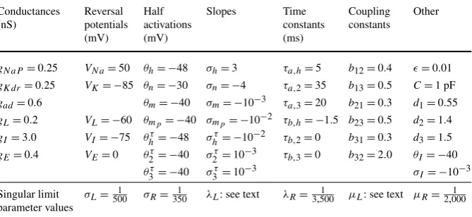
Table 1 Parameter values for full model and singular limit simulations and singular limit analysis corre-sponding to Figure3
Conductances (nS)
Reversal potentials (mV)
Half activations (mV)
Slopes Time
constants (ms)
Coupling constants
Other
gN aP=0.25 VN a=50 θh= −48 σh=3 τa,h=9.5 b12=0.4 =0.01
gKdr=0.25 VK= −85 θn= −30 σn= −4 τa,2=30 b13=0.4 C=1 pF
gad=0.5 θm= −36 σm= −10−1 τa,3=45 b21=0.2 d1=0.21
gL=0.14 VL= −60 θmp= −50 σmp= −10−1 τb,h= −4.5 b23=0.24 d2=0.73
gI=3.0 VI= −75 θhτ= −48 σhτ= −10−2 τb,2= −10 b31=0.3 d3=1.4
gE=0.5 VE=0 θ2τ=0 σ2τ=10−1 τb,3= −32.3 b32=0.25 θI= −32
θ3τ=0 σ3τ=10−1 σI= −10−1
Singular limit parameter values
σL=9501 σR=5001 λL=2,0001 λR=2,0001 μL=1,2701 μR=1,2701
Table 2 Parameter values for full model and singular limit simulations and singular limit analysis corre-sponding to Figures5A and6A
Conductances (nS)
Reversal potentials (mV)
Half activations (mV)
Slopes Time
constants (ms)
Coupling constants
Other
gN aP=0.25 VN a=50 θh= −48 σh=3 τa,h=5 b12=0.4 =0.01
gKdr=0.25 VK= −85 θn= −30 σn= −4 τa,2=35 b13=0.5 C=1 pF
gad=0.6 θm= −40 σm= −10−3 τa,3=20 b21=0.3 d1=0.55
gL=0.2 VL= −60 θmp= −40 σmp= −10−2 τb,h= −1.5 b23=0.5 d2=1.4
gI=3.0 VI= −75 θhτ= −48 σhτ= −10−2 τb,2=0 b31=0.3 d3=1.5
gE=0.4 VE=0 θ2τ= −40 σ2τ=10−3 τb,3=0 b32=2.0 θI= −40
θ3τ= −40 σ3τ=10−3 σI= −10−3 Singular limit
parameter values
σL=5001 σR=3501 λL: see text λR=3,5001 μL: see text μR=2,0001
studies [6,8] and making changes to achieve interesting dynamics; also, we rescaled the capacitanceC to 1 pF and divided all conductances by its original value, 20, correspondingly. Note that the actual values are not important as long as they give a certain nullcline structure and fast-slow time scale separation, as these do (see the general assumptions in Appendix2below).
Note that given(τa,i, τb,i),i=h,2,3, one can compute theσ,λ, and μvalues
that appear in (4), (5), and (6). That is, taking into account thatθ2τ andθ3τ in Table1 are well above the voltages actually achieved in our simulations and thatσhτ<0, we compute the singular limit parameter values in the table as
σL=/τa,h, σR=/(τa,h+τb,h),
μL=/(τa,3+τb,3), μR=/(τa,3+τb,3).
The parameter values listed in Table1for τa,h,τb,h were used during times when
cell 3 was in the active phase and in the subsequent races, whileτa,h=5.75,τb,h= −0.75 were applied during times when cell 4 was active and in the subsequent races; similarly,σLwas changed to 1/575 when cell 4 was active. These values ofτa,h,τb,h
were obtained from preliminary simulations using a slightly different form ofτh(v)
that had been used in earlier studies [6,8, 30], which gave qualitatively identical behavior. This originalτh(v)took different values depending on whether cell 3 or
cell 4 was active becausev1 belonged to different intervals in the two cases. The form ofτh(v)that we adopted, as given in Equation (32), was chosen to unify the
form of the equations across all three neurons and to simplify numerical exploration of parameter space. We note that a change in θmp from −50 to −52 changed the
attractor from 13231323. . . to 132313213. . . as in Figure6A, although this parameter set did not give the full range of patterns seen in the other panels of Figure6.
Similarly, with the values ofθiτ,σiτ,i=h,2,3 given in Table2, the singular limit parameter values in Table2are obtained from
σL=/τa,h, σR=/(τa,h+τb,h),
λL=/(τa,2+τb,2), λR=/τa,2,
μL=/(τa,3+τb,3), μR=/τa,3.
For all panels in Figures 5 and 6, we used the parameter set in Table 2, ex-cept that we adjusted (τa,2, τb,2, τa,3, τb,3) for panels B,C,D. Specifically, we set
(τa,2, τb,2, τa,3, τb,3)to(35,7,20,−3)in Figures5B and6B,(35,10,20,0)in Fig-ures5C and6C, and(35,10,20,−2)in Figures5D and6D.
Appendix 2: General assumptions
System (1) has certain properties that make it suitable for the analysis that we per-form. Given a network of three synaptically coupled elements, our analysis can pro-ceed if the following assumptions on the network and its dynamics are satisfied.
(A1) Each unit in the network consists of a system of two ordinary differential equations (ODE), one for the evolution of a fast variable with anO(1) vec-tor field, call itfj, and one for a slow variable with anO()vector field,sj,
forj∈ {1,2,3}, whereis a small, positive parameter.
(A2) Each unit is coupled to both of the other units in the network. The coupling from unitjto unitkappears as a Heaviside step functionH (fj−θI), or a sufficiently
steep increasing sigmoidal curve with half-activationθI, in the ODE forfk.
(A3) The fast vector field of each unit is a decreasing function of the strengths of the inputs that unit receives. Thus, iffj decreases throughθI, such that the input
from unitj to the other units turns off, thendfk/dtincreases fork=j.
(a) if one input to unitj is on (i.e.,fk> θIfor somek=j), then:
(i) there is a monotone branchNjsilof thefj-nullcline,
(ii) Njsil is defined on an intervalIjsil satisfyingfj< θI for allfj∈Ijsil,
(iii) Njsil intersects thesj-nullcline in a unique point(fj∗, sj∗), and
(iv) (dNjsil(fj)/df )(dsj/dt ) >0 when dsj/dt is evaluated along Njsil
withfj< fj∗;
(b) if no inputs to unitj are on, then:
(i) there is a monotone branchNjactof thefj-nullcline,
(ii) Njact is defined on an intervalIjactsuch thatθI∈Ijact,
(iii) Njactintersects thesj-nullcline in a unique point(fj∗∗, sj∗∗)withfj∗∗< θI, and
(iv) (dNjact(fj)/df )(dsj/dt ) <0 when dsj/dt is evaluated along Njact
withfj> fj∗∗.
For system (1), eachv plays the role of the fast variablef from (A1) while the other variable linked tov is the slow variables. Since S∞(v)is a Heaviside step function, (A2) holds for system (1), and the fact that all coupling is inhibitory, with a reversal potential less than the range of values traversed by eachv, means that (A3) is satisfied as well. Assumption (A4), although more complicated than the others, is in fact fairly standard for typical planar neuronal models. This assumption holds, for example, if a unit’sf-nullcline is the graph of a cubic function for all levels of input; if in the presence of input, the nullcline’s left branch lies belowθI and the unit has a
critical point on this branch; and if in the absence of input, the nullcline’s right branch crosses throughθI, with a critical point on this branch having anf-coordinate less
thanθI. It is easy to choose parameters for the(v1, h)unit in system (1) that meet all of these criteria. The persistent sodium current renders thev1-nullcline cubic, and we can chooseθI and the parameters ofh∞to achieve the other desired properties,
as we do throughout this article. The other two units in the system have monotone
v-nullclines because each can be expressed as a graph(v, m(v))wherem(v)is the ratio of two linear functions ofv. Certain choices ofθIand parameters ofm∞, such as
those made in this article, ensure that (A4) holds for these units as well. We note that the assumptions made about the relations of thef-nullclines toθI can be weakened
as long asfj=θI is only achieved when the inputs to unitj are both off.
Competing interests
The authors declare that they have no competing interests.
Authors’ contributions
JR and DT carried out the analysis, performed the numerical simulations, and wrote the paper.