Sparse Bayesian blind image deconvolution with parameter estimation

R E S E A R C H

Open Access

Sparse Bayesian blind image deconvolution

with parameter estimation

Bruno Amizic

, Rafael Molina

and Aggelos K Katsaggelos

Abstract

In this article, we propose a novel blind image deconvolution method developed within the Bayesian framework. We concentrate on the restoration of blurred photographs taken by commercial cameras to show its effectiveness. The proposed method is based on a non-convexlpquasi norm with 0<p<1 that is used for the image, and a total variation (TV) based prior that is utilized for the blur. Bayesian inference is carried out by utilizing bounds for both the image and blur priors using a majorization-minimization principle. Maximuma posterioriestimates of the unknown image, blur and model parameters are calculated. Experimental results (i.e., restorations of more than 30 blurred photographs) are presented to demonstrate the advantage of the proposed method compared to existing ones.

1 Introduction

Blind image deconvolution (BID) refers to the process of estimating both the original image and the blur from the degraded noisy image observation by using partial infor-mation about the imaging system. Blind image decon-volution algorithms represent a valuable tool that can be used for improving image quality without requiring complicated calibrations of the real-time image acquisi-tion and processing system (i.e., medical imaging, video-conferencing, space exploration, x-ray imaging, etc.).

The blind image deconvolution problem is encountered in many different technical areas, such as astronomical imaging, remote sensing, microscopy, medical imaging, optics, super-resolution applications, and motion track-ing applications among others (see, for example, [1-9]). Astronomical imaging is one of the primary applications of blind image deconvolution algorithms [1,2]. Ground based imaging systems are subject to blurring due to the rapidly changing index of refractions of the atmo-sphere. Extraterrestrial observations of the Earth and the planets are degraded by motion blur as a result of slow camera shutter speeds relative to the rapid spacecraft motion. Blind image deconvolution is used for improv-ing the quality of the Poisson distributed film grain noise present in the blurred X-rays, mammograms, and digital

*Correspondence: [email protected]

1Department of Electrical Engineering and Computer Science, Northwestern University, Evanston, IL, 60208-3118, USA

Full list of author information is available at the end of the article

angiographic images. In such applications, many times, the blurring is unavoidable because the medical imag-ing systems limit the intensity (e.g., low X-ray intensity) of the incident radiation in order to protect the patient’s health [10]. In optics, blind image deconvolution is used to restore the original image from the degradation intro-duced by a microscope or any other optical instrument [6,7]. The Hubble Space Telescope main mirror imper-fections have provided an inordinate amount of images for the digital image processing community [1]. As a final example, in tracking applications the object being tracked might be blurred due to its speed or the motion of the camera. As a result, the track is lost with conven-tional tracking approaches and the application of blind restoration approaches can improve tracking results [9].

The standard formulation of the gray-scale image degra-dation model is given in matrix-vector form by

y=Hx+n, (1)

where theN×1 vectorsx,y, andnrepresent, respectively, the original image, the available noisy and blurred image, and the observation noise, andHrepresents the blurring matrix created from the blur point spread functionh. The images are assumed to be of sizem×n=N, and they are lexicographically ordered intoN×1 vectors. Giveny, the BID problem calls for finding estimates ofxandHusing prior knowledge on them.

A number of methods have been proposed to address BID (a recent literature review can be found in [11]). The most recent methods are based on a Bayesian framework,

and have addressed the removal of the camera motion from blurred photographs [12-19]. In [12] the unknown image and blur were estimated in a two step process. In the first step the blur is estimated from the blurred photo-graph by regularizing the image gradients with a mixture of Gaussian distributions and by regularizing the blur with a mixture of exponential distributions. In the second step the image is estimated from the blurred photograph and the estimated blur by utilizing the Richardson-Lucy (RL) algorithm. Finally, the restored image is obtained by performing the histogram equalization (to that of the observed image) on the output of RL. A multi-scale approach is utilized for the algorithm implementation. The multi-scale approach consists of down-sampling the blurred photograph to number of low resolution images, and by utilizing the proposed algorithm iteratively to obtain the blur estimate at each resolution.

Estimating camera motion has also been investigated in [13,14], where the unknown image and blur were estimated in a simultaneous fashion. Additionally, [14] concentrated on synthetic experiments where the perfor-mance of the algorithm was evaluated by the improvement in signal to noise ratio. Also, in [13,14] the regularization parameters are not automatically estimated but rather heuristically chosen by the user at each iteration in order to yield an unknown image estimate with good visual quality. The major disadvantage of the methods proposed in [13,14] compared to the method proposed in [12] is the lack of parameter estimation.

In this article, we extend our study in [20] by provid-ing (1) a multi-scale based implementation of the algo-rithm which improves the quality of the obtained restored images, and (2) a complete comparison with many exist-ing state of the art blind deconvolution methods. The proposed Bayesian algorithm for BID utilizes a variant of the non-convex lp quasi norm based prior as the

unknown image prior and the TV prior as the unknown blur prior. Furthermore, we utilize the Bayesian frame-work to provide the estimates for all model parameters. Finally, we evaluate the performance of the proposed algorithm and provide comparisons with [12-14,16,19] by restoring blurred photographs taken by commercial cameras.

This article is organized as follows. In Section 2 we provide the proposed Bayesian modeling of the BID prob-lem. The Bayesian inference is presented in Section 3. In Section 4, we describe implementation details of the proposed algorithm. Experimental results are provided in Section 5 and conclusions are drawn in Section 6.

2 Bayesian modeling

As already discussed in the previous section, the observa-tion noise is modeled as a zero mean white Gaussian

ran-dom vector. Therefore, the observation model is defined as

p(y|β,x,h)∝βN/2exp

−β

2 y−Hx

2

, (2)

where β is the precision of the multivariate Gaussian distribution.

As the image prior we utilize a variant of the generalized Gaussian distribution, given by

p(x|α)= 1

ZGG(α) exp

−

d∈D

α_d i

|d_i(x)|p

, (3)

where ZGG(α) is the partition function, 0 < p < 1, α denotes the set {αd} and d ∈ D = {h,v,hh,vv,hv}.

h_i(x) and v_i(x) correspond to, respectively, the hori-zontal and vertical first order differences, at pixeli, that is, h_i(x) = xi − xl(i) and v_i(x) = xi − xa(i), where

l(i) and a(i) denote the nearest neighbors of i, to the left and above, respectively. The operatorshh_i (x),vv_i (x),

hv_i (x) correspond to, respectively, horizontal, vertical and horizontal-vertical second order differences, at pixeli. In this study, similarly to [15,21], we utilize a non-convexlpquasi norm with 0<p<1 since the derivatives

of blurry photographs are expected to be sparse. The dis-tributions of the image derivatives often have heavier tails that are better modeled with the non-convex lp quasi

norm prior with 0<p<1 compared to the convex priors modeled withp=1, 2.

For reducing the complexity of the problem we assume that α_h = α_v = α and α_hh = α_vv = α_hv = α/2. Additionally, similarly to [22], the partition function is approximated asZGG(α)∝α−λ1N/p, whereλ1is a positive real number. We then simplify (3) accordingly to obtain the following image prior

p(x|α)∝αλ1N/p_exp

−α d∈D

21−o(d)

N

i=1

|d_i(x)|p

,

(4)

where o(d) ∈ {1, 2} denotes the order of the difference operatord_i(x).

For the blur we utilize the total-variation prior given by (see [23] for more details)

p(h|γ )∝γλ2N_{exp [}−_{γTV(h)] , (5)}

whereλ2is a positive real number and TV(h)is defined as

TV(h)= i

(h_i(h))2₊₍v

i(h))2. (6)

In this study, we use flat improper hyperpriors onα,β

andγ, that is, we utilize

Note that with this choice of the hyperpriors, the observed imageyis made solely responsible for the estimation of the image, blur and hyperparameters.

3 Bayesian inference

Bayesian inference on the unknown components of the blind image deconvolution problem is based on the estimation of the unknown posterior distribution p(α,β,γ,x,h|y), given by

p(α,β,γ,x,h|y)= p(α,β,γ,x,h,y)

p(y) . (8)

Assuming thatxandhare independent, the joint dis-tribution p(α,β,γ,x,h,y) can be factorized in terms of the observation model p(y|β,x,h), the prior distributions p(x|α)and p(h|γ ), and the hyperparameter distributions p(α), p(β)and p(γ ), that is,

p(α,β,γ,x,h,y)=p(y|β,x,h)p(x|α)p(h|γ )p(α)p(β)p(γ ). (9)

In this study, we adopt the maximum a posteriori (MAP) approach to obtain a single point estimate,¯ = (α¯,β¯,γ¯,x¯,h¯), that maximizes p(α,β,γ,x,h|y)as follows,

¯

=argmaxp(α,β,γ,x,h|y)

=min

β

2y−Hx

2_+α

d∈D

21−o(d)

i

|d_i(x)|p

+γTV(h)−λ1N

p logα− N

2 logβ−λ2Nlogγ . (10)

As can be seen from (10), obtaining the point estimate that maximizes the posterior distribution p(α,β,γ,x,h | y)is not straightforward since it requires the minimiza-tion of a non-convex funcminimiza-tional. Maximizing the posterior distribution p(α,β,γ,x,h|y)by iteratively optimizing in one variable while fixing the others (the so called iterated conditional modes (ICM) method [24]) is equivalent to the variational Bayesian based maximization (see [25] for an example derivation) for the special case when all the posterior distributions are assumed to be degenerate.

In this article, we apply the majorization-minimization approach twice to bound the non-convex functional to be minimized. We start by bounding the non-convex image prior p(x|α)by the functional M1(α,x,Z), that is

p(x|α)≥const· M1(α,x,Z). (11)

The majorization-minimization approach has been uti-lized in several approaches for image restoration [25,26].

The functional M1(α,x,Z)is derived by considering the relationship between the weighted geometric and arith-metic means, which is given by

tp/2z1−p/2≤ p 2t+

1−p

2

z, (12)

wheret≥0,z>0, and 0<p<2. We first rewrite (12) as

tp/2≤ p 2

t+2−_ppz

z1−p/2 . (13)

Using (13) we obtain

|d_i(x)|p≤ p

2

[d_i(x)]2+2−_ppzd,i

z1_d−_,ip/2 . (14)

Therefore, we have

p(x|α)=const·αλ1N/p_exp

−α d∈D

21−o(d)

i

|d_i(x)|p

≥const·αλ1N/p_exp

−αp

2

d∈D 21−o(d)

i

[d_i(x)]2+2−_ppzd,i

z1_d−_,ip/2 ⎤ ⎦.

(15)

Then (11) holds by setting

M1(α,x,Z)=αλ1N/pexp

−αp

2

d∈D 21−o(d)

i

[d_i(x)]2+2−_ppzd,i

z1_d−_,ip/2 ⎤ ⎦,

(16)

where Z is a matrix with elements zd,i, with d ∈ {h,v,hh,vv,hv}andi=1,. . .,N.

Similarly, the majorization-minimization criterion is used to bound the blur prior p(h|γ ) utilizing the func-tional M2(γ,h,u). Let us define, for γ and any N -dimensional vectoru∈ (R+)N, with componentsui, i=

1,. . .,N, the following functional

M2(γ,h,u)=αλ2Nexp

−γ

2

i

(h_i(h))2+(v_i(h))2+ui √

ui

.

(17)

Using the inequality in (13) withp = 1, fort ≥ 0 and z>0, that is,

√

t≤√z+ 1

2√z(t−z), (18)

we obtain

p(h|γ )≥const· M2(γ,h,u). (19)

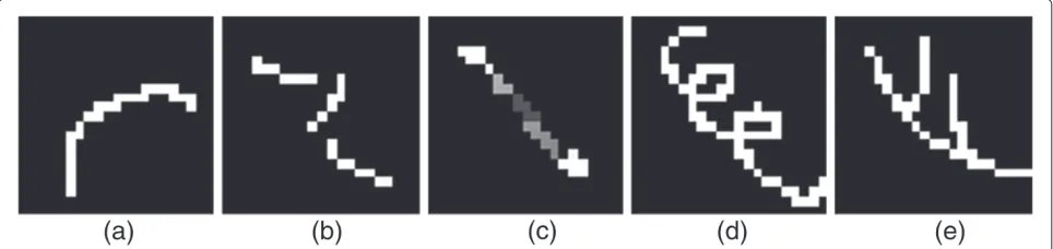
Figure 1Five different synthetic non-parametric motion blurs included in the window of size21×21: (a) Blur 1: the support is14×12, (b)Blur 2: the support is15×14,(c)Blur 3: the support is14×14(d)Blur 4: the support is18×19,(e)Blur 5: the support is18×15.

Table 1 ISNR_ˆxand ISNR_hˆvalues, for the cameraman, satellite, shepp-logan, and airplane images degraded by five different motion blurs (BSNR=40 dB)

Image Blur 1 Blur 2 Blur 3 Blur 4 Blur 5

ISNR_xˆ ISNR_hˆ ISNR_xˆ ISNR_hˆ ISNR_ˆx ISNR_hˆ ISNR_xˆ ISNR_hˆ ISNR_xˆ ISNR_hˆ

cameraman 11.41 20.80 7.07 16.74 6.64 18.41 5.96 21.94 6.92 21.22

satellite 18.50 39.44 17.85 35.49 17.98 20.56 8.76 25.76 9.02 26.17

shepp-logan 32.49 47.34 24.27 45.23 31.16 20.51 22.99 49.00 22.36 49.76

airplane-color 8.10 17.55 9.34 15.67 7.99 15.78 8.50 20.84 4.83 18.32

p(α,β,γ,x,h,y)=p(α)p(β)p(γ )p(x|α)p(h|γ )p(y|β,x,h) ≥const·p(α)p(β)p(γ )M1(α,x,V)M2

(γ,h,u)p(y|β,x,h).

Therefore, a single point estimate that maximizes the lower bound of the posterior distribution p(α,β,γ,x,h | y)is found as follows

¯

=min

β

2y−Hx 2₊αp

2

d∈D 21−o(d)

i

[d_i(x)]2₊2−p p zd,i

z_d1−_,ip/2 +

+γ

2

i

(h_i(h))2+(v_i(h))2+ui

√_u

i

−λ1N

p logα−

N

2 logβ−λ2Nlogγ .

(20)

As shown in (20), we are effectively replacing the origi-nal non-convex minimization problem (10) by a series of convex ones by utilizing the majorization-minimization criteria and introducing the additional variational vectors

zd and u. By iteratively solving this convex optimiza-tion problem in an alternating fashion with respect to all unknowns, we obtain a sequence of point estimates and derive the proposed algorithm as shown next.

3.1 Algorithm

Givenα1,β1,γ1,h1,u1_i =[h_i(h1)]2+[v_i(h1)]2, andz1_d,i. fork=1, 2,. . .until a stopping criterion is met:

1. Calculate

xk=βk(Hk)t(Hk)+αkp

d

21−o(d)(d)tWk_d(d) −1

βk(Hk)ty, (21)

(a)

(b)

(c)

(d)

(e)

(a)

(b)

(c)

(d)

Figure 4Four different original images from [27]: (a) Image 1. (b) Image 2. (c) Image 3. (d) Image 4.

whereWk_dis a diagonal matrix with entries Wk_d(i,i)=(zk_d,i)p/2−1.

2. Calculate

hk+1=

βk(Xk)t(Xk)+γk

d∈{h,v}

(d)tUk(d)

⎤ ⎦

−1

βk(Xk)ty, (22)

whereUkis a diagonal matrix with entries Uk(i,i)=(uk_i)−1/2.

3. For eachd∈ {h,v,hh,vv,hv}calculate

zk_d+_,i1=[d_i(xk)]2, (23)

4. Calculate

uk_i+1=[h_i(hk+1)]2+[v_i(hk+1)]2, (24) 5. Calculate

αk+1 = λ1N/p d∈D21−o(d)

i|di(xk)|p

, (25)

βk+1 = N

y−Hk+1_xk2, (26)

γk+1 = λ2N

TV(hk+1₎, (27)

In the line of study presented in [21] the parameterp is set to 4/5 (see [21] for a detailed discussion). Addition-ally, the parametersλ1andλ2are needed to approximate the partition functions for prior distributions p(x|α)and

p(h|γ ), respectively. Unfortunately, the approximations of partition functions for the distributions p(x|α)and p(h|γ )

are necessary since its corresponding partition functions are analytically intractable. We follow the approaches pro-posed in [22,23], as already described in the previous section, and determine the values of the parameters λ1 andλ2experimentally. The values of the parametersp,λ1, andλ₂ are therefore set throughout all the experiments that follow. The robustness of the proposed method will be tested and evaluated under various blurring and noisy conditions.

Note that if the blurhand the hyperparametersα,β, and

γ are assumed to be known, the proposed algorithm coin-cides with the iteratively re-weighted least squares (IRLS) algorithm presented in [21] (i.e., in this case for both algo-rithms the image estimate is calculated as shown in (21)). Note, that thelpquasi norm based prior is also utilized in

[15], and that this study simplifies the prior used in [21] by omitting the second order derivatives.

4 Multi-scale implementation

The restoration results presented in [12], and more recently in [27], showed the effectiveness of the multi-scale approach in implementing blind image deconvolu-tion algorithms. Furthermore, it is shown in [27] that the multi-scale approach prevents the algorithm from con-verging to the unit impulse. Alternatively, the authors in [13,14] introduced heuristic re-weighting of the reg-ularization parameters, at each iteration, to prevent the

(a)

(b)

(c)

(d)

(e)

(f)

(g)

(h)

Table 2 SSE_xˆand ER_xˆvalues, for the images and blurs defined in Figures 4 and 5, respectively

Blur Method Image 1 Image 2 Image 3 Image 4

SSE_xˆ ER_xˆ SSE_xˆ ER_ˆx SSE_xˆ ER_xˆ SSE_xˆ ER_xˆ

Blur 1 ALG 29.91 0.91 43.93 0.91 24.75 0.78 43.73 1.46

Fergus et al. 39.73 1.21 59.71 1.24 39.48 1.25 44.33 1.48

Cho et al. 33.05 1.00 64.88 1.35 26.74 0.85 31.59 1.05

Shan et al. 49.79 1.51 100.70 2.09 45.83 1.45 53.76 1.79

Levin et al. 44.06 1.34 63.98 1.33 38.82 1.23 78.25 2.61

Blur 2 ALG 33.47 0.89 50.00 0.97 20.59 0.57 42.18 0.96

Fergus et al. 40.70 1.08 66.12 1.29 41.55 1.15 93.14 2.11

Cho et al. 34.13 0.91 53.42 1.04 30.18 0.83 102.24 2.32

Shan et al. 38.87 1.03 313.48 6.11 29.74 0.82 146.73 3.33

Levin et al. 48.50 1.29 74.05 1.44 46.73 1.29 128.82 2.92

Blur 3 ALG 27.45 1.06 19.38 0.45 16.96 0.92 17.78 1.16

Fergus et al. 30.05 1.16 55.75 1.31 21.36 1.16 19.63 1.29

Cho et al. 31.41 1.21 29.17 0.68 17.56 0.95 19.55 1.28

Shan et al. 28.12 1.08 53.48 1.25 19.20 1.04 16.33 1.07

Levin et al. 34.93 1.35 64.27 1.50 18.93 1.03 49.97 3.27

Blur 4 ALG 51.59 1.08 93.70 1.30 28.69 0.74 44.15 1.11

Fergus et al. 125.80 2.64 112.92 1.56 81.28 2.09 11658.02 294.05

Cho et al. 63.73 1.34 80.16 1.11 41.34 1.06 84.32 2.13

Shan et al. 100.43 2.11 178.28 2.47 134.77 3.46 429.12 10.82

Levin et al. 95.81 2.01 105.20 1.45 68.15 1.75 97.73 2.46

Blur 5 ALG 31.39 1.50 36.54 1.32 21.28 1.45 20.27 1.31

Fergus et al. 27.32 1.31 39.50 1.42 21.58 1.47 20.61 1.34

Cho et al. 38.59 1.85 33.25 1.20 23.30 1.59 16.00 1.04

Shan et al. 30.76 1.47 51.94 1.87 17.71 1.21 20.85 1.35

Levin et al. 26.50 1.27 35.98 1.29 17.43 1.19 34.01 2.20

Blur 6 ALG 20.72 1.32 23.71 1.17 18.61 1.88 23.66 1.32

Fergus et al. 44.02 2.80 84.12 4.16 33.29 3.36 46.83 2.62

Cho et al. 42.68 2.72 36.37 1.80 19.24 1.94 37.60 2.10

Shan et al. 71.33 4.54 199.59 9.87 28.90 2.91 58.19 3.25

Levin et al. 28.47 1.81 36.73 1.82 20.98 2.12 62.42 3.49

Blur 7 ALG 38.51 1.90 61.57 1.56 20.74 1.59 64.40 4.36

Fergus et al. 206.70 10.22 152.18 3.86 137.37 10.53 501.31 33.90

Cho et al. 43.46 2.15 48.99 1.24 26.81 2.06 31.38 2.12

Shan et al. 252.56 12.49 250.20 6.34 230.76 17.69 300.06 20.29

Levin et al. 45.91 2.27 64.07 1.62 27.05 2.07 97.97 6.63

Blur 8 ALG 30.07 1.16 44.67 1.10 33.23 1.43 77.69 3.37

Fergus et al. 49.42 1.91 89.65 2.20 51.95 2.24 781.10 33.88

Cho et al. 45.48 1.76 73.35 1.80 47.10 2.03 41.63 1.81

Shan et al. 158.72 6.14 106.66 2.62 202.18 8.73 287.21 12.46

Levin et al. 48.19 1.86 71.32 1.75 31.20 1.35 112.69 4.89

Figure 6Comparing the proposed algorithm with the methods proposed in [12,13,16,19] based on the restoration results from Table 2: Percentage of cases for which the restored image yields the smallest SSE_xˆvalues.

algorithms from converging to unrealistic blur estimates. In our study, no heuristic adjustment of each parame-ter is performed but instead we estimate the parameparame-ters automatically within the Bayesian framework.

To avoid unrealistic blur estimates we adopt here a multi-scale scheme similar in spirit to the one proposed in [12]. Additionally, the proposed multi-scale approach

allows user to automatically initialize the proposed algo-rithm without visually inspecting the observed blurred image for determining the initial blur estimate. By analyz-ing the observed blurred image it is possible to come up with more informative initial blur estimates; however in this study our focus is to develop a completely automated algorithm once the blur support is provided.

The basic idea behind the multi-scale approach is to down-sample the observed blurred image to a number of low resolution images. At the lowest resolution the initial blur estimate (i.e.,h1) is set to the uniform blur and the lowest resolution of the down-sampled observed image is utilized as the initial image estimate (i.e.,x1). After con-vergence is achieved at each scale we up-sample the image and the blur estimates to the next higher resolution and re-run the proposed algorithm. This iterative process is repeated until the algorithm converges and image and blur estimates are obtained at their native resolutions. The detailed pseudocode used in the implementation of our multi-scale approach is shown in Appendix.

5 Experimental results

In this section, we present the experimental results obtained by the use of the proposed algorithm. As the performance metric, for the experiments in which the original image is known, we utilize the improvement in signal to noise ratio of the restored image (denoted as ISNRx_ˆ), which is defined as 10 log10

x−y2_{/x− ˆx}2_,

wherex,yandxˆare the original, observed and estimated images, respectively. Analogously, when the blur is known we utilize the improvement in signal to noise ratio of the restored blur (denoted as ISNR_hˆ), which is defined as 10 log₁₀h−hδ2/h− ˆh2

, whereh,hδandhˆ are

the original blur, the unit impulse, and the estimated blur, respectively.

In addition, after the blur support, greater than the original one, is specified by the user, all unknown param-eters and the estimates of the unknown image and blur

are estimated automatically as described in Sections 3 and 4. Specifying the blur support for the unknown blur is common with the state-of-the-art approaches (see [12-14,16,19]).

Similarly to these approaches, the proposed algorithm is very robust when the support of the blur is largely overestimated by the user, as can be seen in all the exper-iments that follow. Also, for the experexper-iments in which

blurred colored images are considered, only the lumi-nance component of the observed image is restored while the observed chroma components are used to obtain the restored colored image once the original luminance is esti-mated. Finally, the proposed algorithm is terminated when

the criterion xk − xk−1/xk−1 < 10−3 is achieved or the number of iterations reaches 100. After each iter-ation, we enforce the following constraints on the blur estimates: the positivity (blur elements less than zero are set to zero), the support constraint (blur elements

outside of the blur support estimate are set to zero), and the energy conservation (sum of the blur elements equals one).

In the first set of experiments, we evaluate the perfor-mance of the proposed method on four standard images

(cameraman, satellite, shepp-logan phantom and airplane) which are widely used in image restoration experiments. The original images are then blurred with five different motion blurs, which are shown in Figure 1. Realizations of white Gaussian noise are added to the respective blurred

Figure 12Comparing the proposed method with the method proposed in [14]: 1st column represents three different blurred observations, 2nd column represents their respective restorations obtained by the proposed algorithm, 3rd column represents their respective restorations obtained by the method proposed in [14], 4th column represents their respective blurs obtained by the proposed algorithm, 5th column represents their respective blurs obtained by the method proposed in [14].

images in order to obtain degraded images with the blurred signal to noise (BSNR) ratio of 40 dB. The blurred signal to noise ratio is defined as follows

BSNR=10 log₁₀ Var(Hx)

Var(n) , (28)

where Var(·) denotes the variance of the random sequence. Example restorations obtained by the proposed algorithm are shown in Figure 2. The restoration results in terms of the previously defined ISNRx_ˆ and ISNRhˆ,

metrics are shown in Table 1. It can be observed from Table 1 that the proposed algorithm is very robust and it is capable of restoring the blurred images very successfully under various non-parametric motion blurs. Example convergence curves obtained by the proposed algorithm are shown in Figure 3.

In the second set of experiments, we evaluate the performance of the proposed method on a set of 32 blurred test images taken by a commercial camera. The test images are obtained from [27] and they are available online (www.wisdom.weizmann.ac.il/∼levina/ papers/LevinEtalCVPR09Data.zip). The set of 32 blurred

images was obtained by taking the original images shown in Figure 4 and by putting them side by side in order to form a calibration image. Once the calibration image was formed, a commercial camera was mounted on a tripod and eight photos of the calibration image were obtained. Note that during the acquisition process, the Z-axis rotation handle was locked in while the X-axis and Y-axis handles were loosened up in order to simulate in-plane camera shake (see [27] for details; resulting blurs are shown in Figure 5). In this study, we consider a com-parison with the following methods [12,13,16,19]. For convenience, from now on, the methods proposed in [12,13,16], and the best method from [19] will be denoted, respectively, as Fergus et al., Shan et al., Cho et al., and Levin at al., while the proposed algorithm will be denoted as ALG.

The restoration results, for the second set of experi-ments where the original image and blur are both known, in terms of Sum of Squared Errors (i.e., SSEx_ˆ = x− ˆx2) and the SSE ratio test (i.e., ERx_ˆ = SSExˆ/SSEx) defined˜

algorithm is very robust and that it is capable of restoring blurred images taken by a commercial camera very suc-cessfully under various non-parametric motion blurs. In addition, the proposed algorithm is very competitive with the state-of-the-art methods. As can be noted in Table 2, the SSEx_ˆmetric for the proposed algorithm is respectively, on the average, 427, 89, 6, and 21 smaller than the SSEx_ˆ metric for the Fergus at al., Shan at al., Cho at al., and Levin et al. methods. Note that in Fergus’ method, the blur estimation is performed separately from the image estima-tion. In order to understand the differences in the restora-tion results we provide some addirestora-tional informarestora-tion. In Figure 6 it can be seen that for 66 % of tested cases the proposed algorithm yields the smallest SSEx_ˆ values. In addition, Figure 7 shows that for a number of test cases the proposed algorithm is capable of achieving very small ERxˆ

values. For example, there are 78 % of the cases for which the proposed algorithm has ERx_ˆsmaller than 1.5 while at the same time (as the second best) there are 53 % of the test cases for which Cho et al. method achieves such con-dition. Example restorations and comparison with Fergus at al., Cho at al., Shan at al, and Levin at al. are shown, respectively, in Figures 8, 9, 10, and 11.

In the third set of experiments, we compare the perfor-mance of the proposed method with the method proposed in [14] by using the same set of blurred photographs as presented in [14]. Note that in the method proposed in [14] the parameters are not estimated but rather they are manually tuned which results in the sequence of num-bers for each parameter. As can be seen in Figure 12 the restoration results obtained by the proposed algorithm are very competitive with the method proposed in [14]. It is clear from Figure 12 that the proposed algorithm pro-duces much sharper restoration results with higher visual quality. Since we lack the true knowledge of the scene, the comparison metrics SSEx_ˆ and ERxˆ are undefined for this experiment.

6 Conclusions

In this article, a novel blind image deconvolution algo-rithm is presented. The proposed algoalgo-rithm was devel-oped within a Bayesian framework utilizing a non-convex lp quasi norm based sparse prior on the image, and a

total-variation prior on the unknown blur. The proposed algorithm is completely automated once the blur sup-port is provided. Experimental results demonstrate that using sparse priors and the proposed parameter estima-tion, both the unknown image and blur can be estimated with very high accuracy. Furthermore, numerous restora-tions of photographs taken by commercial cameras are provided to demonstrate the robustness and effectiveness of the proposed approach. Finally, it was shown that the performance of the proposed algorithm is competitive

to existing state-of-the-art blind image deconvolution algorithms.

Appendix

Algorithm 1 is shown below.

Competing interests

The authors declare that they have no competing interests.

Acknowledgements

Author details

1_{Department of Electrical Engineering and Computer Science, Northwestern}

University, Evanston, IL, 60208-3118, USA.2_{Departamento de Ciencias de la} Computaci ´on e I.A., Universidad de Granada, 18071 Granada, Spain.

Received: 30 August 2011 Accepted: 4 October 2012 Published: 21 November 2012

References

1. J Krist, inAstronomical Data Analysis Software and Systems IV, ed. by byRA Shaw, HE Payne, and JJE Hayes. Simulation of HST PSFs Using Tiny Tim (Astronomical Society of the Pacific, San Francisco, USA, 1995), pp. 349–353

2. TJ Schultz, Multiframe blind deconvolution of astronomical images. J. Opt. Soc. Am. A.10, 1064–1073 (1993)

3. T Bretschneider, P Bones, S McNeill, D Pairman, inProceedings of the American Society for Photogrammetry & Remote Sensing. Image-based quality assessment of SPOT data, (2001 ). [Unpaginated CD-ROM] 4. FS Gibson, F Lanni, Experimental test of an analytical model of aberration

in an oil-immersion objective lens used in three-dimensional light microscopy. J. Opt. Soc. Am. A.8, 1601–1613 (1991)

5. O Michailovich, D Adam, A novel approach to the 2-D blind

deconvolution problem in medical ultrasound. IEEE Trans. Med. Imaging. 24, 86–104 (2005)

6. M Roggemann, Limited degree-of-freedom adaptive optics and image reconstruction. Appl. Opt.30, 4227–4233 (1991)

7. P Nisenson, R Barakat, Partial atmospheric correction with adaptive optics. J. Opt. Soc. Am. A.4, 2249–2253 (1991)

8. AK RMCA Segall, Katsaggelos, High-resolution images from low-resolution compressed video. IEEE Signal Process. Mag.20(3), 37–48 (2003) 9. S Dai, M Yang, Y Wu, AK Katsaggelos, inProc. IEEE Int Image Processing

Conf. Tracking motion-blurred targets in video, (2006), pp. 2389–2392 10. CJKK Faulkner, M Louka, inThird Int. Conf. on Image Proc. and Its

Applications. Veiling glare deconvolution of images produced by x-ray image intensifiers, (1989), pp. 669–673

11. TE Bishop, SD Babacan, B Amizic, AK Katsaggelos, T Chan, R Molina,Blind Image Deconvolution: Problem Formulation and Existing Approaches. (CRC Press , 2007)

12. R Fergus, B Singh, A Hertzmann, ST Roweis, WT Freeman, Removing camera shake from a single photograph. ACM Trans Graph.25(3), 787–794 (2006)

13. Q Shan, J Jia, A Agarwala, inSIGGRAPH ’08: ACM SIGGRAPH 2008 papers. High-quality motion deblurring from a single image (ACM, New York, 2008), pp. 1–10

14. M Almeida, L Almeida, Blind and semi-blind deblurring of natural images. IEEE Trans. Image Process.19, 36–52 (2010)

15. D Krishnan, R Fergus, inAdvances in Neural Information Processing Systems 22, ed. by Y Bengio, D Schuurmans, J Lafferty, CKI Williams, and A Culotta. Fast image deconvolution using hyper-Laplacian priors, (2009), pp. 1033–1041

16. S Cho, S Lee, Fast motion deblurring. ACM Trans Graph. (SIGGRAPH ASIA 2009).28(5). (Article No. 145, 2009)

17. TS Cho, N Joshi, CL Zitnick, SB Kang, R Szeliski, WT Freeman, inIEEE Conference on Computer Vision and Pattern Recognition (CVPR). A content-aware image prior, (2010), pp. 169–176

18. T Hou, S Wang, H Qin, Image deconvolution with multi-stage convex relaxation and its perceptual evaluation. IEEE Trans. Image Process. 20(12), 3383–3392 (2011)

19. A Levin, Y Weiss, F Durand, W Freeman, inIEEE Conference on Computer Vision and Pattern Recognition (CVPR). Efficient marginal likelihood optimization in blind deconvolution, (2011), pp. 2657–2664 20. B Amizic, SD Babacan, R Molina, AK Katsaggelos, inEuropean Signal

Processing Conference Eusipco. Sparse Bayesian Blind Image Deconvolution with Parameter Estimation (Aalborg, Denmark, 2010), pp. 626–630 21. A Levin, R Fergus, F Durand, WT Freeman, inSIGGRAPH ’07: ACM SIGGRAPH

2007 papers. Image and depth from a conventional camera with a coded aperture (ACM, New York, 2007), p. 70

22. A Mohammad-Djafari, inMaximum Entropy and Bayesian Methods. A full bayesian approach for inverse problems (Kluwer Academic Publishers, 1996), pp. 135–143

23. J Bioucas-Dias, M Figueiredo, J Oliveira, inProceedings of EUSIPCO’2006. Adaptive total-variation image deconvolution: a

majorization-minimization approach (Florence, Italy, p. 2006

24. J Besag, On the statistical analysis of dirty pictures. J. Royal Stat. Soc. Series B (Methodological).48(3), 259–302 (1986)

25. S Babacan, R Molina, A Katsaggelos, Parameter estimation in TV image restoration using variational distribution approximation. IEEE Trans. Image Process.17(3), 326–339 (2008)

26. J Bioucas-Dias, M Figueiredo, J Oliveira, inICASSP, vol. 2. Total-variation image deconvolution: a majorization-minimization approach, (2006), p. II 27. A Levin, Y Weiss, F Durand, WT Freeman, inProc. IEEE Conf. Computer

Vision and Pattern Recognition CVPR. Understanding and evaluating blind deconvolution algorithms, (2009), pp. 1964–1971

doi:10.1186/1687-5281-2012-20

Cite this article as:Amizicet al.:Sparse Bayesian blind image deconvolution with parameter estimation.EURASIP Journal on Image and Video Processing

20122012:20.

Submit your manuscript to a

journal and benefi t from:

7 Convenient online submission

7 Rigorous peer review

7 Immediate publication on acceptance

7 Open access: articles freely available online

7 High visibility within the fi eld

7 Retaining the copyright to your article